Journal of Applied Mathematics and Physics
Vol.06 No.10(2018), Article ID:88034,20 pages
10.4236/jamp.2018.610176
Numerical Investigation by the Finite Difference Method of the Laser Hardening Process Applied to AISI-4340
Rachid Fakir1,2, Noureddine Barka1, Jean Brousseau1, Gabriel Caron-Guillemette2
1Département de mathématiques, informatique et génie, Université du Québec à Rimouski, 300 Allée des Ursulines, Rimouski, QC, Canada
2Bombardier Transport Canada Inc., La Pocatière, Québec, Canada

Copyright © 2018 by authors and Scientific Research Publishing Inc.
This work is licensed under the Creative Commons Attribution International License (CC BY 4.0).
http://creativecommons.org/licenses/by/4.0/


Received: September 24, 2018; Accepted: October 23, 2018; Published: October 26, 2018
ABSTRACT
This paper presents a numerical and experimental analysis study of the temperature distribution in a cylindrical specimen heat treated by laser and quenched in ambient temperature. The cylinder studied is made of AISI-4340 steel and has a diameter of 14.5-mm and a length of 50-mm. The temperature distribution is discretized by using a three-dimensional numerical finite difference method. The temperature gradient of the transformation of the microstructure is generated by a laser source Nd-YAG 3.0-kW manipulated using a robotic arm programmed to control the movements of the laser source in space and in time. The experimental measurement of surface temperature and air temperature in the vicinity of the specimen allows us to determine the values of the absorption coefficient and the coefficient of heat transfer by convection, which are essential data for a precise numerical prediction of the case depth. Despite an unsteady dynamic regime at the level of convective and radiation heat losses, the analysis of the averaged results of the temperature sensors shows a consistency with the results of microhardness measurements. The feasibility and effectiveness of the proposed approach lead to an accurate and reliable mathematical model able to predict the temperature distribution in a cylindrical workpiece heat treated by laser.
Keywords:
Laser Hardening, Scanning Speed, Case Depth, Finite Difference Method, AISI-4340

1. Introduction
Laser surface heat treatment, which aims to improve the properties of materials such as steel and some aluminum alloys, offers many advantages over conventional hardening processes [1] [2] . In this process, the understanding and the precise knowledge of the thermal flows absorbed and reflected by a material is a broad topic that concerns many types of industrial applications. In terms of resistance to wear, fatigue, friction and corrosion, an important part of the research is devoted to surface heat treatment and in particular to selective laser heat treatment [3] . To achieve a good performance in heat treatment, it is necessary to control the case depth generated by the heat flux transmitted by conduction through the outer surface of the workpiece [4] [5] . Several research studies to date have made it possible to present prediction approach techniques of the case depth, to improve the longevity of mechanical parts and to improve understanding of the underlying physics.
T. Miokovic et al. presented in 2006 a study on the superficial hardening of AISI-4140, study based on the effect of inhomogeneous formation of austenite due to conditions of austenization and quenching locally different, and at a dilatometry at high speeds of heating and cooling during the process. Data from this study has been implemented in the ABAQUS finite element program as laws of user-defined materials for a calculation that couples temperature distribution and phase development during heating and cooling process. The results obtained in this study faithfully reproduce the evolution of the temperature as well as the value of the resulting hardness [6] . Michael K.H. Leung et al. presented in 2007 a heat transfer model with a quasi-stable interface for hardening by laser transformation of AISI-1050 steel for a rectangular beam, using IT and CCT diagrams, and with consideration of the initial workpiece temperature, the heating rate and the cooling rate of process. To customize the shape of the rectangular flat-top beam of a conventional Gaussian laser spot beam, a diffractive optical kinoforme (DOK) was used. It has been shown that the theoretical predictions of case depth and hardness concurred perfectly with the experimental results [7] . Ritesh S. Lakhdar et al. presented in 2008 a numerical model that included heat transfer, hardening and tempering for efficient prediction of hardness and phases in temperate zones in a rectangular steel part in AISI-4140 heat treated by overlapping laser beam trajectories. In this study, they combined the developed tempering model with existing models in the literature of thermal behavior and phase change kinetics for the prediction of the three-dimensional profile hardness. The model they developed has been experimentally validated by multitrack laser hardening tests, with optimized parameters providing a case depth of up to 2-mm for an overlap of 5-mm in laser beam trajectories [8] .
Sen-Yung Lee et al. presented in 2014 a new method to solve temperature distribution equations in a workpiece heat treated by laser. The proposed resolution method is based on minimizing the mean squared error between the experimental data obtained and the estimated data of the analytical solution, with time-dependent boundary conditions. The distribution of temperature and heat flux over the entire space-time domain were predicted for real cases to illustrate the simplicity, the effectiveness and precision of the proposed method [9] . Marko Bojinovic et al. presented in 2015a numerical model based on FEM to simulate the laser hardening process of 50CrV4 steel samples. The numerical implementation was possible thanks to the code ABAQUS for laser hardening case studies. The numerical model developed is based on austenitization temperatures (Ac1 and Ac3), on the heating and cooling rate to predict the case depth of the samples. The experimental validation has proven that taking into account the kinetics of the austeniteat a high rate of temperature change is clearly more appropriate [10] . For a determination of the temperature distribution in a material, the finite element method (FEM) can be used to solve numerically the partial differential equations of heat flux in a defined domain and with boundary conditions of Dirichlet, Neumann or Robin [11] . This FEM allows using commercial software to perform simulations on complex geometries by dint of faster resolution of boundary conditions, and with a potentiality of mathematical justifications for convergence and error optimization. Despite its many qualities the FEM remains very complicated to program and requires manipulation by experienced users, because the errors of the users can be fatal for the final solution. And also, because it can be very expensive in memory and in calculation time [12] . However, the finite difference method (FDM) which involves replacing the derivatives of the heat equation by divided differences or a combination of point values in a finite number of discrete points, has the advantage of being simple to write and less expensive in computing time for simple geometries like circular cylinders and plates. The FDM method allows using modeling, to facilitate control of boundary conditions for adjustment of input parameters according time [13] [14] .
In the field of laser heat treatment an interesting but little studied prediction using the finite difference method to predict the temperature distribution inside of a cylindrical workpiece in rotation was developed for a stationary point by the team of R. Fakir et al. in 2018 [15] . Based on a similar and complementary approach, we developed and integrated in this study the focal spot scan parameters at the boundary conditions for efficient prediction of the case depth along the longitudinal axis of the cylinder. The mathematical model was built and validated with experimental tests. The approach was built progressively: 1) by an analysis of the temperature distribution using the heat diffusion equations, the boundary conditions, the properties of the material which depend on the temperature, discretization of the mathematical model by the finite difference method, 2) an experimental validation with a Taguchi experimental design and 3) analysis and discussion of results. The feasibility and effectiveness of the proposed approach lead to an accurate and reliable mathematical model able to predict the temperature profile in a cylindrical workpiece heat-treated with a moving laser source.
2. Thermal Model
2.1. Methodology & Thermal Properties
In this study a mathematical model of laser heat treatment of cylindrical workpiece was developed to predict the temperature distribution and the case depth of the transformation of the microstructure. Figure 1(a) shows the scheme of the experimental setup and Figure 1(b) shows the variation curves for thermal conductivity and specific heat according to the temperature.
The model is based on the calculation of heat flux with an adjustment, by experimental data, of the absorption coefficient of the metal and the coefficient of heat transfer by convection, for a good consideration of the variations of the thermal properties of the material according to the laser heat treatment parameters (including laser beam scanning speed). By means of temperature sensors we measured the evolution of the surface temperature of the cylinder and the surrounding air of the workpiece, according to the laser heat treatment parameters. These temperature measurements were used to estimate the values of the absorption coefficient and the heat transfer coefficient, which are essential data for a good numerical prediction of the case depth related to the eutectoid transformation mechanism. Equations (1) and (2) present the prediction polynomials of the variation of thermal conductivity and specific heat according to the temperature.
(1)
(2)
For the evaluation of the value of the coefficient of heat transfer by convection, we used an empirical correlation adapted to scientific calculations and which groups the dimensionless number Reynolds ( ), Nusselt ( ), and
 (a)
(a) 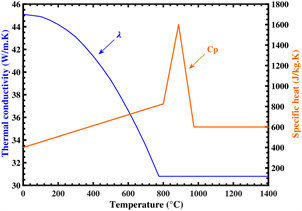 (b)
(b)
Figure 1. Experimental setup: (a) Schematic diagram; (b) Thermal conductivity and specific heat versus temperature.
Prandtl ( ). Equation (3) presents the expression of the empirical correlation for rotating cylinders with a constant rotation speed Ω (rad/s) [16] . Equation (4) presents the empirical correlation giving the value of the coefficient of heat transfer by convection according to the thermal conductivity of the air, the diameter of the cylinder, the rotation speed of the cylinder, the kinematic viscosity of air and the thermal diffusivity of air. This equation is valid only for and .
(3)
(4)
For the estimation of the value of the heat transfer coefficient through the empirical correlation of Equation (4) it is necessary to know the exact values of the thermo-physical properties of the air (κ, β and γ) in the vicinity of the cylindrical workpiece. Properties that were determined by experimental trials and that are dependent of laser heat treatment parameters (laser power, scanning speed and rotational speed of the cylindrical part).
2.2. Heat Conduction Equation in Cylindrical Coordinates
The quantity of power density of the Gaussian beam I(x, y) transmitted by conduction in the workpiece, is modeled based on the heat conduction Equation (5) for a revolution system with an axial temperature gradient depending on the time.
(5)
Equation (6) presents the transversal profile in the space of the Gaussian laser beam that propagates in the direction of the z-axis [17] .
(6)
With and , the coordinates defining the center of the laser beam. P is the maximum value of I(x, y) measured at the center defined by and .
2.3. Initial Condition and Boundary Conditions
The initial temperature of the cylinder is supposed to be uniform Tin = 27˚C. This initial condition makes it possible to determine the coefficients which are solutions of the equations of the system at the beginning of the laser heat treatment (at t = 0 s). The laser beam moves from the start-laser position (reference position x = 10-mm) to stop-laser position (end position of the course x = 40-mm) with a constant scanning speed SS. The sample is continuously rotating on a test bench with a fixed rotation speed Ω. The diameter of the focal spot of the laser beam is set at 0.50-mm. Equation (7) shows the expression of the course distance of the focal spot at time t and according to the average scanning speed of the course.
(7)
Boundary conditions are expressed according to equation 8, for a good consideration of the scanning speed of the laser beam and starting and stopping positions at the outer surface of the cylinder (r = R).
(8)
Equation (9) presents the expression of the boundary conditions outside and inside the zone irradiated by the laser beam. The first term of condition 1 represents convective heat losses and the second term represents the heat losses by radiation. The first term of condition 2 represents the amount of energy transmitted by the laser beam to the workpiece and the second term represents thermal losses by convection and radiation.
(9)
3. Numerical Model (FDM)
3.1. Discretization of Model Equations
Finite difference method [18] allows through Taylor developments to search the approximate solutions of partial derivatives of heat transfer equations [19] . Equations (10)-(13) present a discretization of the terms of equation 5 with an explicit schema using the finite difference method. In chronological order, the first term corresponds to the first derivation of the temperature according to the radius (r), the second term corresponds to the first derivative of the temperature according to the time (t), the third term corresponds to the second derivation of the temperature according to the radius (r) and the last term corresponds to the second derivation of the temperature according to the x-axis of rotation of the cylinder. and represent respectively the mesh size along the radial axis and the axis of rotation, and the pitch of the temporal mesh.
(10)
(11)
(12)
(13)
Equation (14) presents the expression of the temperature, at the moment t + dt according to the value of the temperature at time t, by means of an explicit discretization of the Fourier-Kirchkoff equation.
(14)
The initial temperature of the cylinder is assumed to be constant T(i, j, 0) = 27˚C. Equations (15) and (16) present a discretization with an explicit finite difference scheme of conditions 1 and 2 of Equation (9). This represents the boundary conditions outside and inside the area irradiated by the laser beam, during its course at a scanning speed SS.
Condition 1: où
(15)
Condition 2:
(16)
Equation (17) shows, a simplified writing of the 4th-order polynomials for solving the equations of conditions 1 and 2. The prediction of the value of the temperature T(R, j, t) on the surface of the cylindrical workpiece can be done by applying the numerical method of Regula Falsi, which consists of repeating the interval division to find the value of T(R, j, t) solution of conditions 1 and 2.
(17)
Ψ, Π, and Γ, are the respective coefficients of the monomials of degree 4, 1 and 0.The laser energy is zero (I = 0) in the term Γ corresponding to the condition 1.
(18)
(19)
(20)
Figure 2 shows a summary algorithm of the thermal model for predicting the distribution of the temperature at any point belonging to the cylindrical workpiece. The input data of the algorithm are: The thermal properties of the material, the dimensions of the cylinder and the parameters of the laser heat treatment (laser power, focal spot diameter, scanning speed and rotational speed of the cylindrical workpiece).
3.2. Mesh Stability Study
The numerical solution of the partial differential equations of the thermal model was done by the finite difference method. The method requires a convergence study of the mesh to ensure a stability of the numerical scheme, a consistency between the exact solution and the discretized solution and finally a convergence of the results of the thermal model [20] . The Lax-Wendroff theorem informs that a numerical scheme converges when the spatio-temporal mesh is very small, that is when , and . As, a refined mesh

Figure 2. Master resolution algorithm for predicting temperature distribution according to the laser heat treatment parameters.
provides more accurate results with a considerable calculation time (important and not insignificant),it is necessary to carry out a manual convergence study of the mesh to optimize the parameters: computing time, data storage memory and accuracy of output results. A study that consists of creating a mesh using a reasonable number of elements, followed by an analysis of the output results, then a slight increase in the mesh density and an analysis of the results by comparison with the results of the previous iteration. This study of manual convergence of the mesh allows us to obtain a precise and exact solution with a sufficiently dense mesh and without requiring too many computing resources. Equation (21) presents, for an explicit numerical scheme in finite differences (Equation (14)), the condition of convergence that connects the pitch of the temporal mesh with the pitch of the spatial mesh and .
(21)
Figure 3 shows the value of the temperature according to the number of meshes, for a point on the surface of the cylinder, at a distance of 15-mm from the laser heat treatment start point, and for a scanning speed of 10-mm/s and a rotation speed of 5000-RPM.The convergence of the mesh has been obtained for approximately 37,500 mesh elements. Which corresponds to a spatial-temporal mesh m and s.
4. Experimental Validation
4.1. Experimental Setup and Experimental Design
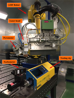
The experimental tests were carried out on specimens of cylindrical geometry in steel AISI-4340, with a diameter of 14.5-mm and a length of 50-mm. Figure 4(a) shows a visualization of the experimental setup, which is composed mainly of a laser source Nd: YAG de 3.0-kW (IPG YLS-3000-ST2) and an articulated robot 6-DOF supporting the laser head. The trajectory of the laser beam, is perpendicular to the axis of rotation of the workpiece to harden. The specimen fixation

Figure 3. Temperature versus number of elements for P = 2800-W.
 (a)
(a) (b)
(b) (c)
(c)
Figure 4. (a) Experimental setup. Hardness curve versus depth; (b) For 3000-W and 6000-RPM; (c) For 2800-W and 4000-RPM.
is ensured by a rotating test rig which can reach 10,000-RPM and which is equipped with a central support with three jaws and a counter-head moving along the x-axis. To measure the surface temperature of the workpiece according to the laser heat treatment parameters, a MI-IGAR-12-LO pyrometer and a FLIR thermal infrared camera with a sensitivity of less than 5˚C, and which can cover a temperature range up to 2000˚C, have been exploited. Four J-type precision thermocouples with a sensitivity of 0.05-s were placed in the vicinity of the cylindrical part to evaluate the ambient air temperature according to the laser heat treatment parameters, by using a NI-USB-6009 which offers features data acquisition (DAQ).Before laser heat treatment, the samples were heat-treated in the oven to homogenize the hardness value. The oven heat treatment consisted of placing the samples in an oven at a 900˚C austenitization temperature for a period of 20-min, followed by cooling in the oil and tempering in the oven at a temperature of 650˚C for a period of 100-min to obtain a uniform hardness of 25-HRC (Rockwell C) [21] . After laser heat treatment, the samples were carefully prepared, cut, coated, polished and etched using a Nital chemical solution (95% ethanol and 5% nitric acid). The hardness profiles were characterized by microhardness measurements programmed using the Clemex machine.
To perform experimental modeling, it is essential to have relevant tests to adequately represent the desired results. The acquisition of validation results with a reasonable number of tests requires the definition of an ordered sequence of experimental tests using an experimental design. Experiment planning based on the Taguchi method optimizes the number of tests to be performed while maintaining the robustness, performance and statistical consistency of a factor design [22] . In the case of laser heat treatment of cylindrical workpieces, it is important to avoid the melting of the surface layer of the material while having a transformation of this same superficial layer. Experimental tests begin with the definition of the minimum and maximum values of the experimental design factors, that are in the case of this study: laser power, scanning speed, and rotation speed. Figure 4(b) and Figure 4(c) show the results of the preliminary tests for measuring the microhardness according to the laser heat treatment parameters.
Table 1 presents the 3 factors at 3 levels considered in the planning of the experiments. The levels of the experimental plan were chosen in the preliminary tests to correspond with the minimum transformation (100-μm) and the maximum transformation (250-μm) of the cylindrical workpiece, which respectively correspond to the laser hardening parameters of the test 9 (2800-W, 10-mm/s and 5000-RPM) and test 1 (3000-W, 8-mm/s and 4000-RPM). Table 2 shows the grid of tests according to the matrix L9 Taguchi, with the results of measurement of the case depth, values of the dimensionless numbers (Reynolds and Prandtl), the thermal conductivity of the air and the absorption coefficient of the material. L9 matrix output responses were determined by examining the hardness profile by measuring the microhardness, the surface temperature and the air temperature around the workpiece by using an infrared camera and air temperature

Table 1. Factors and levels of experience planning.
Table 2. L9 orthogonal matrix and experimental results.
sensors. We note that the thermal conductivity of the air, the Reynolds and Prandtl numbers are proportional to the laser power and the rotation speed of the cylinder and are inversely proportional to the scanning speed of the laser beam. With a maximum difference of about 0.36E−02 W/m-K for the thermal conductivity of the air, of 347 for the Reynolds number and a small difference of about 0.008 for the Prandtl number. And that the absorption coefficient is proportional to the scanning speed and inversely proportional to rotational speed and laser power, for a difference of about 0.074 between the maximum laser hardening configuration and the minimum configuration.
4.2. Analysis of Results and Discussion
To estimate the value of the convective heat transfer coefficient and the absorption coefficient according to the laser power, the scanning speed and the rotation speed, an ANOVA analysis of variance with the general step-by-step method, detailed in Table 3 and Table 4, was performed [23] . The factor with the lowest contribution rate, which corresponds to the level of significance α = 0.05, was put in error factor compared to all the conditions of interaction between the parameters.
For each process parameter, the value of the variance ratio F was compared with the values of the standard F tables for high statistical significance levels. It was concluded that the heat transfer coefficient is mainly linked with the rotation speed Ω, for a model response value of about 98%. And that the absorption
Table 3. ANOVA table for h.
Table 4. ANOVA table for Λ.
coefficient depends mainly on the two factors P and SS, for a model response value of about 94%. Equations (22) and (23) present the empirical prediction relationships, of the heat transfer coefficient and the absorption coefficient, on the basis of a linear regression.
(22)
(23)
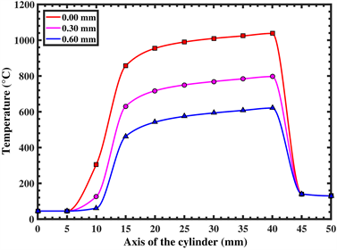
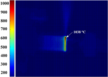
Figure 5(a) and Figure 5(b) show the estimated response surfaces [24] for the heat transfer coefficient and the absorption coefficient, according to the laser power, the scanning speed and the rotation speed. These response surfaces of the statistical model make it possible to reproduce the contour lines with response intervals varying according to laser heat treatment parameters. Response surfaces were represented according to dimension less numbers: Reynolds, Prandtl and the dimensionless variable reproduced following the Buckingham approach [25] to reduce the number of response surfaces of the statistical model. The constant α = 9549 was introduced to convert the SI system to the engineering system: the scanning speed from m/s to mm/s and the rotation speed from rad/s to RPM. It can be deduced from the figures obtained that a high rotational speed increases the convective losses but also allows to increase the value of the absorption coefficient for the levels of the factors experimental design (P, SS and Ω) presented in Table 1. The results obtained confirm that the value of the hardness is proportional to the laser power and the rotation speed, and is inversely proportional to the scanning speed. Figure 5(c) and Figure 5(d) show the temperature distribution along the x-axis of the cylinder for three depths and with different laser heat treatment parameters. Figure 5(e) and Figure 5(f) show
 (a)
(a)
 (b)
(b)
 (c)
(c)
 (d)
(d)
 (e)
(e)
 (f)
(f)
Figure 5. Contour plot: (a) For h; (b) For Λ. Temperature versus Axis of the cylinder; (c) For 2800-W, 10-mm/s and 5000-RPM; (d) For 3000-W, 8-mm/s and 6000-RPM. Infrared thermography for the laser parameters; (e) Configuration (c); (f) Configuration (d).
the comparison values of the surface temperature at the stop-laser position (40-mm) using an infrared camera with an emittance coefficient of 0.123 and a distance between the camera lens and the cylinder surface of about 700-mm. Visualization with the thermal camera allowed us to give identical surface temperature values for a constant emissivity coefficient and this regardless of the laser heat treatment parameters. At the start position of the laser heat treatment (10-mm), the surface temperature rapidly increases from 27˚C to about 300˚C in 50-ms.Then from the 10- to 15-mm position, it rises from 300˚C to about 850˚C, followed by a slight increase every 5-mm of displacement.
This slight increase in temperature between the position 15-mm and 40-mm is due to the heating phenomenon by advancement and can be explained by the fact that the thermal properties (thermal conductivity and specific heat)change with the temperature, and that convection and radiation heat losses become more important for high temperatures. This phenomenon induces a slight modification of the case depth along the longitudinal of the cylinder. To remedy this, it’s important to control the laser heat treatment parameters being processed.
The transformation start temperature allows us to estimate the case depth to improve the mechanical performance of the sample. The AISI-4340 steel used has an initial allotropic transformation temperature of 727˚C (Ac1), a complete austenitization temperature of about 927˚C (Ac3), and a melting temperature of about 1417˚C. To validate the developed model, it was assumed that the depth reaching a complete austenitization temperature (Ac3) will have a martensitic microstructure if the rate of the cooling cycle is greater than 8˚C/s. Figure 6(a) shows the heating cycle for laser heat treatment parameters corresponding to the test 9 (Table 2), with the values of the temperature for three depths and at the position 25-mm. It is observed for the parameters of the test 9, that the temperature Ac3 is obtained for a depth of 100-μm. Figure 6(b) shows the heating cycle for the laser heat treatment parameters corresponding to test 1 at the same position 25-mm. It is observed for the parameters of the test 1, that the temperature Ac3 is obtained for a depth of 250-μm. The variation of the temperature from 27˚C to 1038˚C, from the moment t = 0 s which corresponds to the position 10-mm to the moment t = 1.5 s which corresponds to the position 25-mm for a scanning speed 10-mm/s (test 9), and from 27˚C to 11,878˚C, from the moment t = 0 s to t = 1.857 s which corresponds to the position 25-mm for a scanning speed 8-mm/s (test 9), is related to the scanning speed of the laser beam, the variation of the thermal properties according to the temperature, the thermal losses and the high concentration of the laser energy in a very small section of the focal spot [26] .
Figure 6(c) and Figure 6(d) show respectively the cooling cycles corresponding to the heating cycles of Figure 6(a) and Figure 6(b) at the same position 25-mm. We observe that the temperature drops quite rapidly after passing the laser beam and this because of the modes of heat transfer by convection and radiation. Compared with Time-Temperature-Transformation (TTT) curves of AISI-4340 steel, we can deduce conclusions about microstructure-scale transformation. As can be seen in Figure 6(c) and Figure 6(d), the cooling rate is of the order of 20˚C/s at the core of the workpiece. This cooling rate is higher than the critical speed (8˚C/s), which is the minimum cooling speed of steel AISI-4340
 (a)
(a)
 (b)
(b)
 (c)
(c)
 (d)
(d)
 (e)
(e)
 (f)
(f)
Figure 6. Temperature versus heating time for three depth and at x = 25-mm: (a) 2800 W, 10 mm/s and 5000RPM; (b) 3000 W, 8 mm/s and 6000 RPM. Temperature versus cooling time; (c) 2800 W, 10 mm/s and 5000 RPM; (d) 3000 W, 8 mm/s and 6000 RPM; (e) Radial hardness profile; (f) Case depth measured versus predicted.
[27] requiring the formation of a completely martensitic structure. Figure 6(e) shows a cross-section of the hardened area, for two configurations of the laser heat treatment parameters, and a microscopic visualization with magnification (×1000) of the microstructure of the transformed zone. The magnification of the zone transformed by the laser heat treatment shows a completely martensitic structure. Figure 6(f) illustrates measurement values of case depth for the position 25-mm, by interpreting the results provided by our model that predicts the temperature value based on the Ac3 transformation temperature and according to laser power, scanning speed and rotation speed.
These results confirm that the mathematical model developed is accurate in predicting temperature during heating and cooling. The temperature values predicted by the model fit well with the case depth measured using the Clemex® microhardness machine. The developed model provides comparable results in the parameter range of Table 1, with a difference of less than 5% compared to the experimental tests.
5. Conclusions
In this study, the temperature distribution in a cylindrical workpiece heat treated by laser was simulated using the finite difference method. The major findings are summarized below:
The algorithm developed with the FDM model for AISI-4340 steel, by adding the displacement parameter of the laser beam, is very effective in simulating the temperature distribution in a workpiece heat treated by laser. The results of theoretical predictions correspond to the experimental tests.
The variation of the thermal properties of the material has been integrated so as not to affect the output results of the thermal model. The coefficient of convective heat transfer has been evaluated by empirical correlations using measurements of the air temperature around the cylinder. Measurements provided by precision thermocouples that have been positioned very close to the outer surface of the cylinder.
The variation of the absorption coefficient that influences the effective penetration of heat flux, according to interaction conditions between the laser energy and the workpiece surface was approximated using experimental tests based on Taguchi experience planning and ANOVA analysis of variance.
Experimental validation of the model by the use of an infrared camera confirmed the values of the predicted temperature on the surface, in the range of defined parameters by the experimental design.
It would be interesting to consider completing this model of prediction of the temperature profile, by integrating a control of the laser heat treatment parameters for a uniform case depth along the longitudinal axis of the cylinder. We believe that this type of approach is the most appropriate way to develop a prediction model of the case depth for workpieces of cylindrical geometry.
Conflicts of Interest
On behalf of all authors, the corresponding author states that there is no conflict of interest.
Cite this paper
Fakir, R., Barka, N., Brousseau, J. and Caron-Guillemette, G. (2018) Numerical Investigation by the Finite Difference Method of the Laser Hardening Process Applied to AISI-4340. Journal of Applied Mathematics and Physics, 6, 2087-2106. https://doi.org/10.4236/jamp.2018.610176
References
- 1. Komanduri, R. and Hou, Z.B. (2001) Thermal Analysis of the Laser Surface Transformation Hardening Process. International Journal of Heat and Mass Transfer, 44, 2845-2826. https://doi.org/10.1016/S0017-9310(00)00316-1
- 2. Senthil Selvan, J., Subramanian, K. and Nath, A.K. (1999) Journal of Materials Processing Technology, 91, 29-36. https://doi.org/10.1016/S0924-0136(98)00430-0
- 3. Suárez, A., Amado, J.M., Tobar, M.J., Yánez, A., Fraga, E. and Peel, M.J. (2010) Study of Residual Stresses Generated inside Laser Cladded Plates Using FEM and Diffraction of Synchrotron Radiation. Surface & Coatings Technology, 204, 1983-1988. https://doi.org/10.1016/j.surfcoat.2009.11.037
- 4. Wang, J.-T., Weng, C.-I., Chang, J.-G. and Hwang, C.-C. (2000) The Influence of Temperature and Surface Conditions on Surface Absorptivity in Laser Surface Treatment. Journal of Applied Physics, 87, 3245-3258. https://doi.org/10.1063/1.372331
- 5. Tobar, M.J., álvarez, C., Amado, J.M., Ramil, A., Saavedra, E. and Yánez, A. (2006) Laser Transformation Hardening of a Tool Steel: Simulation-Based Parameter Optimization and Experimental Results. Surface & Coatings Technology, 200, 6362-6367. https://doi.org/10.1016/j.surfcoat.2005.11.067
- 6. Miokovic, T., Schulze, V., Vohringer, O. and Lohe, D. (2006) Prediction of Phase Transformations during Laser Surface Hardening of AISI 4140 Including the Effects of Inhomogeneous Austenite Formation. Materials Science and Engineering A, 435-436, 547-555. https://doi.org/10.1016/j.msea.2006.07.037
- 7. Leung, M.K.H., Manb, H.C. and Yu, J.K. (2007) Theoretical and Experimental Studies on Laser Transformation Hardening of Steel by Customized Beam. International Journal of Heat and Mass Transfer, 50, 4600-4606. https://doi.org/10.1016/j.ijheatmasstransfer.2007.03.022
- 8. Lakhkar, R.S., Shin, Y.C. and Krane, M.J.H. (2008) Predictive Modeling of Multi-Track Laser Hardening of AISI 4140 Steel. Materials Science and Engineering A, 480, 209-217. https://doi.org/10.1016/j.msea.2007.07.054
- 9. Lee, S.-Y. and Huang, T.-W. (2014) A Method for Inverse Analysis of Laser Surface Heating with Experimental Data. International Journal of Heat and Mass Transfer, 72, 299-307. https://doi.org/10.1016/j.ijheatmasstransfer.2013.12.067
- 10. Bojinovic, M., Mole, N. and Stok, B. (2015) A Computer Simulation Study of the Effects of Temperature Change Rate on Austenite Kinetics in Laser Hardening. Surface and Coatings Technology, 273, 60-76. https://doi.org/10.1016/j.surfcoat.2015.01.075
- 11. Cheng, A.H.-D. and Cheng, D.T. (2005) Engineering Analysis with Boundary Elements. Engineering Analysis with Boundary Elements, 29, 268-302. https://doi.org/10.1016/j.enganabound.2004.12.001
- 12. Bathe, K.-J. and Wilson, E.L. (1976) Numerical Methods in Finite Element Analysis. Vol. 197, Prentice-Hall, Englewood Cliffs, NJ.
- 13. Wang, B.-L. and Tian, Z.-H. (2005) Application of Finite Element–Finite Difference Method to the Determination of Transient Temperature Field in Functionally Graded Materials. Finite Elements in Analysis and Design, 41, 335-349. https://doi.org/10.1016/j.finel.2004.07.001
- 14. Fakir, R., Barka, N. and Brousseau, J. (2018) Optimization of the Case Depth of a Cylinder Made with 4340 Steel by a Control of the Laser Heat Treatment Parameters. ASME 2018 International Design Engineering Technical Conferences and Computers and Information in Engineering Conference, Quebec City, 26-29 August 2018, 1-9.
- 15. Fakir, R., Barka, N. and Brousseau, J. (2018) Case Study of Laser Hardening Process Applied to 4340 Steel Cylindrical Specimens Using Simulation and Experimental Validation. Case Studies in Thermal Engineering, 11, 15-25. https://doi.org/10.1016/j.csite.2017.12.002
- 16. Bergman, T.L. and Incropera, F.P. (2011) Fundamentals of Heat and Mass Transfer. John Wiley & Sons, Hoboken.
- 17. Khosrofian, J.M. and Garetz, B.A. (1983) Measurement of a Gaussian Laser Beam Diameter through the Direct Inversion of Knife-Edge Data. Applied Optics, 22, 3406-3410. https://doi.org/10.1364/AO.22.003406
- 18. Smith, G.D. (1985) Numerical Solution of Partial Differential Equations: Finite Difference Methods. Oxford University Press, Oxford.
- 19. Richtmyer, R.D. and Morton, K.W. (1994) Difference Methods for Initial Value Problems. 2nd Edition, Krieger Publishing, Malabar.
- 20. Aziz, A.K. (1972) The Mathematical Foundations of the Finite Element Method with Applications to Partial Differential Equations. Academic Press, Cambridge, 796.
- 21. Fakir, R., Barka, N. and Brousseau, J. (2018) Mechanical Properties Analysis of 4340 Steel Specimen Heat Treated in Oven and Quenching in Three Different Fluids. Metals and Materials International, 24, 981-991. https://doi.org/10.1007/s12540-018-0120-9
- 22. Ross, P.J. (1988) Taguchi Techniques for Quality Engineering. McGraw-Hill, New York.
- 23. Palanikumar, K., Karunamoorthy, L., Karthikeyan, R. and Latha, B. (2006) Optimization of Machining Parameters in Turning GFRP Composites Using a Carbide (K10) Tool Based on the Taguchi Method with Fuzzy Logics. Metals and Materials International, 12, 483-491. https://doi.org/10.1007/BF03027748
- 24. Myers, R.H. (1971) Response Surface Methodology. Allyn and Bacon, Boston.
- 25. Buckingham, E. (1914) On Physically Similar Systems. Illustrations of the Use of Dimensional Equations. Physical Review, 4, 345-376.
- 26. Soltani, P. and Akbareian, N. (2014) Finite Element Simulation of Laser Generated Ultrasound Waves in Aluminum Plates. Latin American Journal of Solids and Structures, 11, 1761-1776. https://doi.org/10.1590/S1679-78252014001000004
- 27. Thelning, K.-E. (1984) Steel and Its Heat Treatment, Butterworth-Heinemann. 2nd Edition, Elsevier, New York, 696.
Nomenclature
Λ Absorption coefficient of the material,
Cp Specific heat, J∙kg−1∙K−1,
h Thermal transfer coefficient, W∙m−2∙K−1,
k Thermal conductivity of the air, W∙m−1∙K−1,
λ Thermal conductivity of steel, W∙m−1∙K−1,
σ Stefan-Boltzmann constant, W∙m−2∙K−4,
ϕs Diameter of the laser spot, m,
D Diameter of the cylinder, m,
γ Thermal diffusivity, m2∙s−1,
ε Emissivity of material surface,
L Cylinder length, m,
nt Number of temporal mesh nodes,
ρ Density, kg∙m−3,
nr Number of mesh nodes following R,
nx Number of mesh nodes following X,
Nu Nusselt’s number,
Pr Prandtl’s number,
Re Reynolds number,
ζr Pitch of the spatial mesh following R, m,
ζx Pitch of the spatial mesh following X, m,
ζt The pitch of the temporal mesh, s,
P Laser power, W,
I Efficient laser power, W,
SS Scanning speed, mm/s,
R Radius of the cylinder, m,
Cd Case depth, μm,
l(t) Spatiotemporal position of beam, m,
T∞ Ambient air temperature, ˚C,
Ac1 Heating temperature at point A1, ˚C,
Ac3 Heating temperature at point A3, ˚C,
T Temperature of the material, ˚C,
Tin Initial material temperature, ˚C,
β Kinematic viscosity, m2∙s−1,
Ω Rotation speed of the cylinder, RPM,
r Distance from laser beam centre, m,
r0 Laser beam radius, m.