Open Journal of Business and Management
Vol.03 No.03(2015), Article ID:58336,18 pages
10.4236/ojbm.2015.33032
Analysing and Optimising Bank Real Estate Portfolio by Using Impulse Response Function, Mahalanobis Distance and Financial Turbulence
Ognjen Vukovic
Department for Finance, University of Liechtenstein, Vaduz, Liechtenstein
Email: ognjen.vukovic@uni.li, oggyvukovich@gmail.com
Copyright © 2015 by author and Scientific Research Publishing Inc.
This work is licensed under the Creative Commons Attribution International License (CC BY).
http://creativecommons.org/licenses/by/4.0/


Received 21 June 2015; accepted 25 July 2015; published 28 July 2015
ABSTRACT
This paper analyses one of the main factors that cause financial crisis and that are real estate portfolio management in banks. VAR and SVAR models were introduced and impulse response functions were obtained. The aforementioned function demonstrated how residential prices reacted to shock. Afterwards, financial turbulence index based on Mahalanobis distance and correlation between real estate prices in Austria, Germany and Switzerland was calculated and its relation to stock prices in EURO area. Financial turbulence demonstrated the lagging effect of financial crisis originating from USA. Data were taken from St. Louis FED database. Having calculated correlations, portfolio was created consisting of REITs, ETFs and stocks. It was optimised and efficient frontiers were found for different portfolio weightings. It was proved that the best way to optimise real estate portfolio was to invest in Swiss real estate as prices were growing and to hedge with Austrian real estate or some variations of ETFs.
Keywords:
Mahalanobis Distance, Real Estate, Portfolio Management, Financial Turbulence, Impulse Response Function, Germany, Switzerland, Austria, Portfolio Optimisation, Efficient Frontier, Correlation

1. Introduction
Financial bubbles are a real threat to the system. The arousal of financial bubbles must be closely monitored as there is a possibility to cause havoc in financial systems. In order to analyse the financial bubbles, nonlinearities and illogical movement of correlated time series must be observed. One of the newly introduced tools in the aforementioned time series analysis is impulse response functions.
Impulse response function demonstrates how the endogenous variables react to shock through time. Although impulse response functions are related to SVAR and VAR models, their observation independently can be very useful as they serve as a perfect tool to observe illogical movement between time series. By observing impulse response functions, it could come to a conclusion that illogical movement could act as a predictor of real estate bubbles. If the link between real estate movement and other macroeconomic variables is broken, it could be said that variables start to follow random walk which is characteristic in the financial theory. At the same time, if variables are correlated in the way that economic and financial theory cannot explain, then the threat of the financial contagion and financial crisis is high. Impulse response functions are based on SVAR models. The basic idea behind impulse response functions is the following: As SVAR model represents an econometric model, it describes the evolution of a set of
 variables over the same sample period. At the same it has the error term that is represented like
 . Impulse response function tries the following. It “shocks” the error term or in the other words, it refers to the reaction of any dynamic system in response to some external change. It is used to show how the financial systems or the variables that are observed react to exogenous impulses, which usually are called by economists as a “shock”.
After having introduced VAR and SVAR models, impulse response function will be introduced. The results of impulse response function for Austria, Germany and Switzerland will be presented. The results will be analysed and will be tried to be applied to real estate portfolio management by analysing correlation between stock prices and real estate price movement in the aforementioned countries. After careful analysis, the portfolio consisting of REITS and leading stock indices, EFTs, will be tried to be optimised and efficient frontier will be found. Concerning the aforementioned analysis, sensitivity analysis will be conducted and different points of efficient frontier will be obtained.
2. Background and Theory
2.1. VAR Model, Lyapunov Exponent and Martingale
Firstly VAR [1] models will be introduced.
VAR model is used to detect interdependencies in the linear interdependent model. It has the following formation:
 (1)
(1)
where the l-periods back observation yt−l is called the l-th lag of y, c is a k × 1 vector of constants (intercepts), Ai is a time-invariant k × k matrix and et is a k × 1 vector of error terms. The thing that must be noted is that all variables must be of the same order of integration. The order of integration denoted
 is the number of differences required to obtain a covariance stationary series. In statistics, a stationary process is defined as a stochastic process whose joint probability distribution does not change when shifted in time. Consequently, parameters do not change over time and do not follow any trends.
The stationary process [2] is defined in the following way:
Formally, let
 be a stochastic process and let
 represent the cumulative distribution of the joint distribution function of
 at times
 . Then
 is said to be strictly (or strongly) stationary if, for all
 , for all
 and for all
 , the following equation is valid:
 (2)
(2)
Since
 doesn’t affect
 is not function of time.
Covariance stationary series means that covariance is stable or in the other words not changing over time. However series that we are observing are martingale series, which means that they do not exhibit covariance dependency. Martingale is defined in the following way:
In the probability theory, a martingale [3] is a model of a fair game where knowledge of past events never helps predict the mean of future winings. In particular, a martingale is a sequence of random variables (stochastic process) for which, at a particular time in the realized sequence, the expectation of the next value in the sequence is equal to the present observed value even given knowledge of all prior observed values. An unbiased random walk (in any number of dimensions) is an example of a martingale.
It is defined in the following way:
A basic definition of a discrete-time martingale [4] as a discrete-time stochastic process for a sequence of random variables
 that satisfies for any time n,
 (3)
(3)
The conditional expected value of the next observation, given all the past observations, is equal to the last observations. Due to the linearity of expectation, this second requirement is equivalent to:
 (4)
(4)
or
 (5)
(5)
For our analysis, the time series that we observe are Markovian time series and martingale processes that follow Brownian motion. Figure 1 shows and demonstrates graphically stopped Brownian motion as an example of martingale because those are the time series we will observe.
One of the theorems will be used. The theorem states that:
T.1. One of the continuous martingale process with stationary increments is Brownian motion. (Hamilton et al. 1994) [3] .
At the same time there exist other martingale processes [5] but it is assumed that those processes are not observed. In this way, VAR model functions really well and impulse response function can be observed.
The variables that we are observing are the following:
1) Inflation;
2) Commercial and construction estate prices;
3) GDP;
4) Real estate prices.
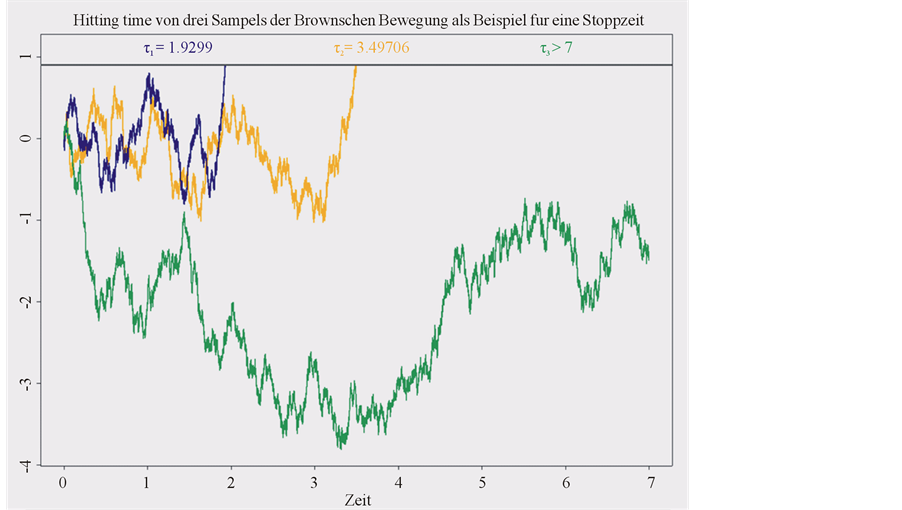
Figure 1. Stopped Brownian motion as an example of martingale. Author own calculation.
Howitt and Clower demonstrate that economic systems emerge spontaneously on their own from a decentralized state [6] . As the whole economics generally comes in cycles, it is necessary to see whether or not randomness contributes to increasing or decreasing oscillations. Not all randomness is regular Brownian motion (RBM). Most is not regular Brownian motion, but is the special type of fractal Brownian motion (FBM) where the fractal dimension is 0.5 (Sanderson, 2009). In order to analyse the data, the Sanderson plot [7] will be taken. Figure 2 demonstrates the prepolicy attractor before European Central Bank implemented crisis measures.
This prepolicy attractor, shown in Figure 2, demonstrates that there is no steady random state for any observed variable as we see that attractors are wide spread and they don’t demonstrate any fixed point. After implementing the stage three of ECB policy, the situation is still chaotic. The attractor shows that the
 state compared to the
 has no defined movement.
The following post-policy attractor [7] shown in Figure 3 demonstrates the situation after crisis measures.
After implementig the policy, the situation is still chaotic as however there is more regularity, but not even that much to be a deterministic process.
In order to explain the behavior of the system, Lyapunov exponent [8] will be used as it can describe the randomness of the system.
Lyapunov exponent is defined in the following way:
 (6)
(6)
where
 is the Lyapunov exponent.

Figure 2. Prepolicy attractor (before ECB implemented crisis measures) [7] .

Figure 3. Postpolicy attractor [7] .
In mathematics, the Lyapunov exponent is a quantity that characterizes the rate of separation of infintensimally close trajectories. MLE is a maximum Lyapunov exponent which determines the notion of predictability for a dynamical system. A positive MLE says that the system is chaotic. On the other side, the system demonstrates that it is dissipative if MLE is negative. Dissipative means that system is operating far from equilibrium and that time series in that case cannot be predicted. Although the policy has caused the system to start orbiting around the point, but is doing so in a random FBM manner.
According to [7] , MLE is before policy −0.0234 and after the policy, it is −0.0985. It means that the aforementioned systems are exhibiting randomness and this supports martingale hypothesis.
Therefore we are talking about local martingale that is a subclass of martingale.
It can be shown that attractor policy of ECB is given in the graph below that is shown in Figure 4.
Figure 4 demonstrates attractor point for European Central Bank policy.
It is shown that equilibrium point can be achieved, but oscillation around the equilibrium point is not predictible. This supports our hypothesis of local martingale and covariance stationarity, therefore VAR and SVAR model can be introduced.
2.2. SVAR Model
Now the SVAR models will be introduced. From an economic point of view, if the joint dynamics of a set of variables can be represented by a VAR model, then the structural form is a depiction of the underlying, “structural”, economic relationships [1] . Two features of the structural form make it the preferred candidate to represent the underlying relations:
・ Error terms are not correlated.
・ Variables can have a contemporaneous impact on other variables.
Structural VAR model is defined with the following equation:
 (7)
(7)
Because of the parameter identification problems, SVAR models cannot be estimated by using ordinary least squares method, but they can be solved by using reduced VAR models. Cholesky decomposition takes one of the leading factors in reducing VAR models using lower- or upper-triangular matrix. Cholesky is a matrix decomposition that ensures that your residual covariance matrix could be transformed into a diagonal matrix. The purpose of this Cholesky decomposition is that the impulse to one variable (or their innovations) must be unrelated to the impulse in another variable, otherwise, it is unrealistic to assume that one variable would remain static (no impulse) while the other moves (impulse).
2.3. Impulse Response Function
Impulse response function [9] is widely used in signal processing. It demonstrates the response of the dynamical

Figure 4. Attractor point for ECB policy, no stable state, oscillation around point [7] .
function to the external signal. In economics impulse response functions are used in order to analyse how the function reacts to exogenous shocks. IRF are used to track the response of a system’s variables to impulses of the system’s shocks. Orthogonalising the VAR’s shocks is required so that the shocks tracked by IRFs are uncorrelated. Combining the needs of identification and non-arbitrary orthogonalisation has since become the focus of structural VAR (SVAR) analysis. We use the short-run SVAR model with two lags per variable.
However IRF are not perfect. They typically suffer from large small-sample biases stemming from bias in the estimated autoregressive coefficients. On the other side, they give a good demonstration how the system that is covariance stationary, in the other words system whose covariance matrix is not changing, reacts to shocks.
2.4. Mahalanobis Distance and Financial Turbulence
After having introduced the external aspect of the analysis, the Mahalanobis distance [10] will be analysed and its relation to financial turbulence.
Mahalanobis distance is introduced as
 (8)
(8)
The Mahalanobis distance is the distance of an observation
 from a group of observations with mean
 and covariance matrix S. Mahalanobis distance is ideal for the portfolio management as it is multivariate, unitless and scale-invariant and it takes into consideration the correlations between the variables. The aforementioned distance will be used in analysis of the financial turbulence index. It represents a multivariate measure of dispersion. It can be shown in the diagram below:
Figure 5 which is shown above demonstrates graphically the derivation of Mahalanobis distance. Firstly multivariate data is given, secondly coordinate system pertaining to the data is constructed and according to Chebyshev

Figure 5. Construction of Mahalanobis distance. Source: Author’s own graph.
inequality, ellipse is obtained. Next the data is transformed to Descartes system and dispersion is measured according to Mahalanobis distance formula. Mahalanobis distance demonstrates the distance of every data point from the center of ellipse. It is a multi-dimensional generalization of the idea of measuring how many standard deviations is the point away from the mean of distribution.
2.5. Financial Turbulence
Financial turbulence describes the volatility of the model as well as its complexity [11] . It will be graphically presented and analysed. The analysis is conducted in the R environment by using ROC curves and Mahalanobis distance. ROC curve is a receiver operating characteristic curve. It helps measure the performance of different models through a visual chart that makes the analysis very statistical friendly. Besides the graph, the accuracy of the model can be assessed measuring the area under the ROC curve. An area of 1 represents a perfect test, an area of 0.5 represents a worthless test, the random guessing procedure. So the closer to the 1 AUC, the better model. This measure is close to Gini coefficient.
After having introduced the impulse response function and financial turbulence index, the correlation between Germany, Austrian and Swiss real estate prices will be compared. Correlation will be calculated as well as the correlation between stock prices in Europe, USA and real estate prices in the European area. Afterwards, the following correlations will be tried to be connected to impulse response functions. In order to analyse portfolio, code in R was written where the combination of real estate investment trusts in Germany, Switzerland and Austria are pooled with the leading stock indices in the aforementioned countries. The efficient frontier is obtained and the optimal point on the aforementioned frontier. Sensitivity analysis is conducted in order to obtain possible portfolio points and to find the best possible portfolio. Code will be given in the Appendix.
3. Methodology and Modeling
3.1. IRF Austria
The following impulse response function was applied to the following equations:
VAR Model―Substituted Coefficients:
===============================
CONSTRUCTION_AUSTRIA = - 0.25058940696*CONSTRUCTION_AUSTRIA(-1) - 0.459750115918*CONSTRUCTION_AUSTRIA(-2) - 0.114121589618*CONSUMER_AUSTRIA(-1) + 0.130215108021*CONSUMER_AUSTRIA(-2) + 0.00190293002625*RESIDENTIAL_AUSTRIA(-1) + 0.00240637865452*RESIDENTIAL_AUSTRIA(-2) + 0.185136772789
CONSUMER_AUSTRIA = - 0.637860667041*CONSTRUCTION_AUSTRIA(-1) + 1.16688027213*CONSTRUCTION_AUSTRIA(-2) + 1.0320494548*CONSUMER_AUSTRIA(-1) - 0.0389801786987*CONSUMER_AUSTRIA(-2) - 0.00141428580892*RESIDENTIAL_AUSTRIA(-1) + 0.024944905185*RESIDENTIAL_AUSTRIA(-2) + 0.576676354912
RESIDENTIAL_AUSTRIA = - 0.703620433172*CONSTRUCTION_AUSTRIA(-1) - 0.246400501023*CONSTRUCTION_AUSTRIA(-2) - 0.766625066844*CONSUMER_AUSTRIA(-1) + 0.900406609385*CONSUMER_AUSTRIA(-2) + 0.405273848586*RESIDENTIAL_AUSTRIA(-1) + 0.0786561614292*RESIDENTIAL_AUSTRIA(-2) - 10.5826435239
Figure 6 demonstrates Impulse response functions which are included in SVAR model for Austria real estate prices. Every variable is considered endogenous and two lags of the variables were taken according to Akaike Information Criterion [12] . It can be seen that the reaction of construction prices to residential prices is not strong, almost with no change at one s.d. Consumer prices are increasing with residential prices, while the cooling of the system can be seen for the shocks to the lags of residential prices in Austria to current residential prices, so there is no risk of financial crisis. At the same time, consumer Austria prices are stable. The system of Austria seems to be stable, the Lyapunov exponent is zero, it means that system is not changing, so there is no problematic issue.
3.2. IRF Germany and Switzerland
Next country that will be considered is Germany.

Figure 6. Impulse response function for Austria. Source: Own calculations.
The equations are given below:
VAR Model―Substituted Coefficients:
===============================
CONSTRUCTION_BIS = 1.04015622893*CONSTRUCTION_BIS(-1) - 0.010605943681*CONSTRUCTION_BIS(-2) - 0.113103992437*CONSTRUCTION_BIS(-3) + 0.0599629558709*CONSTRUCTION_BIS(-4) + 0.172399894059*INDUSTRIAL_BIS(-1) - 0.0629487441808*INDUSTRIAL_BIS(-2) - 0.0538620378999*INDUSTRIAL_BIS(-3) + 0.0768575005362*INDUSTRIAL_BIS(-4) - 0.121412907321*INFLATION_BIS(-1) - 0.183074076281*INFLATION_BIS(-2) + 0.217417409139*INFLATION_BIS(-3) - 0.037264304489*INFLATION_BIS(-4) + 0.0953327936089*RESIDENTIAL_BIS(-1) - 0.240315699426*RESIDENTIAL_BIS(-2) + 0.231742731516*RESIDENTIAL_BIS(-3) - 0.0791813608327*RESIDENTIAL_BIS(-4) + 1.15881032878
INDUSTRIAL_BIS = - 0.0565084568727*CONSTRUCTION_BIS(-1) - 0.0157230991653*CONSTRUCTION_BIS(-2) + 0.227748482533*CONSTRUCTION_BIS(-3) - 0.0756151355205*CONSTRUCTION_BIS(-4) + 1.68516154854*INDUSTRIAL_BIS(-1) - 1.10257422148*INDUSTRIAL_BIS(-2) + 0.365193713622*INDUSTRIAL_BIS(-3) - 0.0511688446375*INDUSTRIAL_BIS(-4) + 0.147883781154*INFLATION_BIS(-1) + 0.103473341741*INFLATION_BIS(-2) + 0.0625277406773*INFLATION_BIS(-3) - 0.31406140906*INFLATION_BIS(-4) - 0.0293426026949*RESIDENTIAL_BIS(-1) + 0.112594480255*RESIDENTIAL_BIS(-2) - 0.0956294175642*RESIDENTIAL_BIS(-3) + 0.0309590164752*RESIDENTIAL_BIS(-4) + 0.429794861285
INFLATION_BIS = - 0.0503339307518*CONSTRUCTION_BIS(-1) + 0.0780212358795*CONSTRUCTION_BIS(-2) + 0.172509321418*CONSTRUCTION_BIS(-3) - 0.18807452317*CONSTRUCTION_BIS(-4) + 0.195038273478*INDUSTRIAL_BIS(-1) - 0.359851587789*INDUSTRIAL_BIS(-2) + 0.335509872932*INDUSTRIAL_BIS(-3) - 0.132303998713*INDUSTRIAL_BIS(-4) + 0.740482791169*INFLATION_BIS(-1) + 0.198040117272*INFLATION_BIS(-2) - 0.245682150704*INFLATION_BIS(-3) + 0.242074891337*INFLATION_BIS(-4) - 0.0405214313903*RESIDENTIAL_BIS(-1) + 0.173648666406*RESIDENTIAL_BIS(-2) - 0.197100290085*RESIDENTIAL_BIS(-3) + 0.0670286912536*RESIDENTIAL_BIS(-4) + 1.5064426254
RESIDENTIAL_BIS = - 0.313697913637*CONSTRUCTION_BIS(-1) + 0.273689944471*CONSTRUCTION_BIS(-2) + 0.0422829641854*CONSTRUCTION_BIS(-3) - 0.219963030411*CONSTRUCTION_BIS(-4) - 0.324385842268*INDUSTRIAL_BIS(-1) + 0.302938398084*INDUSTRIAL_BIS(-2) + 0.284481595201*INDUSTRIAL_BIS(-3) - 0.194853688117*INDUSTRIAL_BIS(-4) + 0.402197862793*INFLATION_BIS(-1) - 0.168427186612*INFLATION_BIS(-2) - 0.283674858661*INFLATION_BIS(-3) + 0.277947523561*INFLATION_BIS(-4) + 1.92903825032*RESIDENTIAL_BIS(-1) - 1.18149247039*RESIDENTIAL_BIS(-2) + 0.397777336912*RESIDENTIAL_BIS(-3) - 0.190296911198*RESIDENTIAL_BIS(-4) - 3.06061094373
Figure 7 demonstrates Impulse response functions which are included in SVAR model for German real estate prices. The four lags were used according to Akaike information criterion. It looks that shock to all the variables except real estate are increasing. The connection between variables are broken, which doesn’t represent a problem if we consider time series as local martingales. But if the time series are dependent, real estate prices can foreshadow the possible financial contagion and crisis.
The Switzerland exhibits increasing real estate prices. Figure 8 demonstrates impulse response function for Swiss real estate market. At the same time, other variables are constant and they are moving without any connection. It is proved that correlation between variables is random or that there is according to Sanderson (2012) there is no correlation. This satisfies the system.
3.3. Financial Turbulence
After having analysed one aspect of real estate, next analysis will follow financial turbulence [13] . By using Mahalanobis distance and ROC curve, financial turbulence is calculated. It is presented in the graph below.
Financial turbulence is demonstrated in Figure 9, which exposes volatility of portfolio of real estate prices, that the biggest shock of the crisis was felt in 2011 for the aforementioned countries, where the distance from the mean was around 40 standard deviations which is based on Mahalanobis distance .In the whole, it means that the crisis is lagging in the aforementioned countries and it is still present because the financial turbulence index has a value of 13,367 that is still high. In the next graph autocorrelation of financial turbulence will be given.

Figure 7. Impulse response function for Germany residential. Source: Own calculation.

Figure 8. Impulse response function of Swiss real estate market. Source: Own calculation.

Figure 9. Financial turbulence (volatility and percentage change) of port- folio of real estate prices of Germany, Austria and Switzerland. Source: Own calculation.
Figure 10 demonstrates the autocorrelation of financial turbulence.
Autocorrelation exhibits non importance of lags therefore it confirms that the aforementioned series follows random walk and stationarity of series is confirmed. The autocorrelation is defined in the following way (Priestley M.B. et al. 1981):
 (9)
(9)
where
 is the expected value operator. The autocorrelation must lie between 1 and −1. The biggest correlation is at 10th lag which means that process is lagging 2 - 3 years which explains financial turbulence.
After having analysed the impulse response function and financial turbulence, the correlation between real estate prices and stock prices will be given. The data is taken from St. Louis FED. The residence price as a time-series is given in the following graph, taking 1970 as the index year and concerning Austria, because of lack of data, the 2000 is taken as index year. The graph of residence price movement in Switzerland, Germany and Austria is given in Figure 11. Figure 11 at the same time demonstrates the comparison of residence prices in these three countries.
Correlation between German and Swiss prices is 0.98, so it means they are perfectly well correlated. Impulse response function demonstrates that Swiss real estate prices will continue to grow, but however German growth is slowing down, therefore the implication is the following:
Although the correlation between German and Austrian real estate prices will decrease, the correlation is still too high to make investment as a measure of diversification in the aforementioned real estate in Germany and Switzerland.
However the correlation between residence prices in Austria and Germany and Austria and Switzerland is around 0.4. Therefore there is still positive correlation, so investing in real estate portfolio in those countries and by examining impulse response functions, it can be seen that growth of German real estate prices are positively correlated with Austrian real estate prices which means that investing in German and Austrian real estate can be defined as that growth of real estate prices in Germany causes also growth in real estate Austrian prices. But if we analyse the real estate management, not from a correlational perspective, because Pearson correlation coefficient indicates the strength of linear relationship between two variables, but its value does not completely characterize their relationship. The graph shows that real estate prices in Austria are stable and will stay stable according to impulse response function, while the real estate prices in Germany are growing, therefore investment in those real portfolios is the following:
If you want to hedge, invest most of the real estate portfolio in Austrian real estate as it is stable and bet according to impulse response function that German real estate prices will continue to grow and then they will be characterised by a drop. That is the point when the bank or investor should sell the real estate portfolio in Germany.

Figure 10. Autocorrelation of financial turbulence. Source: Own calculation.

Figure 11. Residence price in Switzerland, Germany and Austria [14] .
When it comes to real estate prices in Switzerland and Austria, the portfolio can be more diversified by investing in Austrian real estate and Swiss real estate. Swiss real estate demonstrates that the prices will continue to grow, therefore portfolio in banking can be more diversified and more money can be invested in Swiss real estate and less in Austrian, because Austrian real estate imply stability, but as it is certain that Swiss real estate market will continue to grow, investment in Swiss real estate will secure certain profit.
In order to proceed, the correlation between EURO area stock prices and real estate prices in Germany and Switzerland will be analysed. Firstly, the stock prices movement in EURO area will be presented in Figure 12 which is shown below.
Correlation between EURO area stock prices and Germany real estate prices is −0.49 until 2000. Afterwards the aforementioned correlation reduced to −0.33. This implies the following:
In order to hedge the portfolio, the best option is to invest in German or Swiss real estate and part of the funds should be directed into European stock prices. In that way, the portfolio can be hedged.
The correlation between EURO area stock prices and Switzerland real estate prices is −0.04. Hedging possibilities are much lower here.
In order to conclude the aforementioned section, the movement of USA stock prices as well as comparison between real estate prices in Germany and USA will be given in Figure 13 and is shown below.
Figure 14 demonstrates the comparison between movement of USA real estate prices and residence prices in Germany. It is followed that residence price in Germany are lagging behind the USA real estate prices. It should also be noted that financial contagion is the consequence of real estate price movement in USA and that the effect of movement of German real estate price is lagging.
The following issues will be observed in portfolio optimisation procedure in the following chapter.
4. Portfolio Optimisation
The portfolio that we made is composed of the following:
・ PSP Swiss Property AG is a Switzerland based real estate holding company. It is assumed that its stock price is the reflection of real estate prices in Switzerland.

Figure 12. Stock prices EURO area [14] .

Figure 13. Real estate USA [14] .

Figure 14. Comparison between USA real estate prices and German residence price. Source: Author’s own calculation.
・ TAG Immobilien AG (TEG) is a real estate company based in Germany whoe activities include the acquisition, development as well as the management of residential real-estate. The company focus lies on the German real-estate market, especially on regions such as Hamburg, Berlin, Munich. TAG is a proprietor of approximately 75,000 residential units and realises appreciation potential within its portfolio through active asset management and strategic acquisition of attractive properties. TAG Immobilien stock price reflects the price movement of German real estate market.
・ Deutsche Wohnen AG, through its subsidiaries acquires, develops and manages residential properties in Germany. Its property portfolio comprises approximately 149,000 residential and commercial units.
・ As there are no REIT companies in Austria, they are traded on stock exchange, we will take the VOESTALPINE AV company which produces concrete and steel and that is related to housing industry. If more real estates are built, more will be invested and share price will grow. But if the price is stable, as it is in Austria, there will be no big need for additional real estate, so the stock price will be stable.
For stock, we will take ETF that invest in stocks.
Firstly, we will take iShares MSCI Germany ETF (EWG). It is a passive ETF that seeks to replicate MSCI Germany index. The index measures the performance of the German equity market.
The other ETF we will take is iShares MSCI Austria Capped ETF, named EWO. It seeks to track the investment results of a broad-based index composed of Austrian equities.
EWL is iShares MSCI Switzerland Capped ETF. It is a passive ETF that seeks to replicate MSCI Switzerland Index.
So the above mentioned assets are taken and inserted into the portfolio optimisation code as inputs.
At first try portfolio is equally distributed among all assets, only 10% is invested in Austrian VOESTALPINE AV company.
First case:
“PSPN” = 0.15, “TEG” = 0.15, “DWNI” = 0.15, “EWG” = 0.15, “EWO” = 0.15, “EWL” = 0.15, “VOE” = 0.10.
Figure 15 demonstrates the optimisation of portfolio for weights presented in Case 1.
Considering the portfolio constructed in this way, it is obvious we are not at the optimal point as risk is too high while return is too low. Now we can try the following combination of investing more in Swiss real estate, less in German and mild amount in Austrian.
Figure 16 demonstrates the optimisation of portfolio for weights in the second portfolio.
For the second portfolio, the situation is better. We already have put more weight in the Swiss real estate investment trusts because we are aware that prices will continue to grow and in order to hedge one part was invested in ETF in Austria. The graph above was obtained. It has higher Sharpe ratio and higher return. It must be noted that return is based on week basis.

Figure 15. Efficient frontier and optimal portfolio for Case 1. Source: Author’s own calculation.

Figure 16. Efficient frontier and optimal portfolio―Case 2.
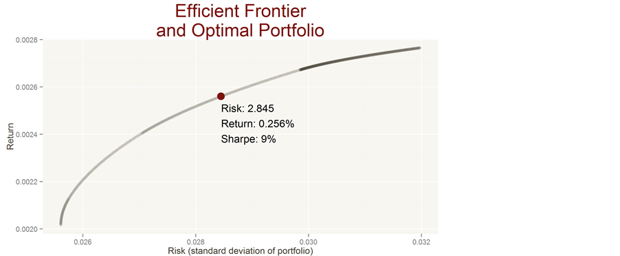
Figure 17. Investment in real estate portfolio completely in Swiss real estate.
If the biggest part is invested in Swiss real estate property, the following situation is obtained:
Figure 17 demonstrates the optimal portfolio if the investment is completely directed in Swiss real estate.
The Sharpe ratio is higher as well as return and risk. In order to optimise portfolio, the R code for portfolio optimisation will be given in the appendix, so that the reader of the paper can experiment with the aforementioned portfolio.
5. Conclusions
After having introduced VAR and SVAR models and index of financial turbulence, the real estate market in Germany, Switzerland and Austria was analysed. By using impulse response function, the possible movement of real estate prices was presented in the aforementioned countries. In order to analyse the movement of real estate prices in connection to stock price movement, correlations have been calculated between real estate prices in Germany, Switzerland and Austria. At the same time, correlations between real estate prices and stock prices in aforementioned countries were calculated. In order to analyse portfolio decisions, possible investment strategies in different assets were proposed. In the end, portfolio optimisation was proposed. Pool of assets that was included comprised REITs and ETFs from Germany, Switzerland and Austria. At the end, R code was given so the reader could mimic the portfolio optimisation construction. The conclusion is that negative correlation between European area stocks and real estate prices in Germany, Switzerland and Austria represents a good hedging opportunity during the financial crisis. As Austria real estate prices are stable, it is possible to hedge by investing in Austrian real estate market and risking part of the portfolio by investing in Swiss real estate market. Possibilities are vast and depending from the risk aversion of the investor; it can be decided how the investment can be conducted.
The index of financial turbulence demonstrated that financial crisis of 2008 that originated in USA, had a lagging effect on Europe which proved that the banks didn’t learn the lessons from the crisis or the lessons were only partially learnt. New models were proposed that could help capture and predict the future financial crisis. Author of this paper sincerely hopes that proposed models will help banks to construct better models to capture the movement and better monitor the movement of real estate stock market.
Acknowledgements
I would like to thank my family and colleagues for immense support while writing the paper.
Cite this paper
OgnjenVukovic, (2015) Analysing and Optimising Bank Real Estate Portfolio by Using Impulse Response Function, Mahalanobis Distance and Financial Turbulence. Open Journal of Business and Management,03,326-344. doi: 10.4236/ojbm.2015.33032
References
- 1. Pfaff, B. (2008) VAR, SVAR and SVEC Models: Implementation within R Package vars.
- 2. Hamilton, J.D. (1994) Time Series Analysis. Princeton University Press, Princeton, 293.
- 3. Hamilton, J.D. (1994) Difference Equations. Time Series Analysis. Princeton University Press, Princeton, 5.
- 4. Williams, D. (1991) Probability with Martingales. Cambridge University Press, Cambridge. http://dx.doi.org/10.1017/CBO9780511813658
- 5. Dung, N.T. and Thao, T.H. (2010) An Approximate Approach to Fractional Stochastic Integration and Its Application.
- 6. Howitt, P. and Clower, R. (2000) The Emergence of Economic Organization. Journal of Economic Behavior & Organization, 41, 55-84. http://dx.doi.org/10.1016/S0167-2681(99)00087-6
- 7. Sanderson, R. (2013) Does Monetary Policy Cause Randomness or Chaos? A Case Study from the European Central Bank. A Case Study from the European Central Bank. Banks and Bank Systems, 8, 55-61.
- 8. Priestley, M.B. (1981) Spectral Analysis and Time Series. Academic Press, Waltham.
- 9. Lütkepohl, H. (2008) Impulse Response Function. The New Palgrave Dictionary of Economics. 2nd Edition. http://dx.doi.org/10.1057/9780230226203.0767
- 10. Stöckl, S. and Hanke, M. (2013) Financial Applications of the Mahalanobis Distance.
- 11. Gonçalves, C.P. (2012) Financial Turbulence, Business Cycles and Intrinsic Time in an Artificial Economy. Algorithmic Finance, 1, 141-156. http://dx.doi.org/10.2139/ssrn.2002698
- 12. Hacker, R.S. and Hatemi, J.A. (2008) Optimal Lag-Length Choice in Stable and Unstable VAR Models under Situations of Homoscedasticity and ARCH. Journal of Applied Statistics, 35, 601-615. http://dx.doi.org/10.1080/02664760801920473
- 13. Rebonato, R. (N.D.) Theory and Practice of Model Risk Management.
- 14. St. Louis FED Website. https://www.stlouisfed.org
Appendix
(http://economistatlarge.com/portfolio-theory/r-optimized-portfolio)
R code for portfolio optimisation
# Economist at Large
# Modern Portfolio Theory
# Use solve.QP to solve for efficient frontier
# This file uses the solve.QP function in the quadprog package to solve for the
# efficient frontier.
# Since the efficient frontier is a parabolic function, we can find the solution
# that minimizes portfolio variance and then vary the risk premium to find
# points along the efficient frontier. Then simply find the portfolio with the
# largest Sharpe ratio (expected return / sd) to identify the most
# efficient portfolio
install.packages ('stockPortfolio')
install.packages('ggplot2')
install.packages('reshape2')
install.packages('quadprog')
library(stockPortfolio) # Base package for retrieving returns
library(ggplot2) # Used to graph efficient frontier
library(reshape2) # Used to melt the data
library(quadprog) #Needed for solve.QP
# Create the portfolio using ETFs, incl. hypothetical non-efficient allocation
stocks <- c(
"PSPN" = 1,
"TEG" = 0,
"DWNI" =0,
"EWG" = 0,
"EWO" = 0,
"EWL" = 0,
"VOE" =0
)
# Retrieve returns, from earliest start date possible (where all stocks have
returns <- getReturns(names(stocks[-1]), freq="week") #Currently, drop index
#### Efficient Frontier function ####
eff.frontier <- function (returns, short="no", max.allocation=NULL,
risk.premium.up=.5, risk.increment=.005){
# return argument should be a m x n matrix with one column per security
# short argument is whether short-selling is allowed; default is no (short
# selling prohibited)max.allocation is the maximum % allowed for any one
# security (reduces concentration) risk.premium.up is the upper limit of the
# risk premium modeled (see for loop below) and risk.increment is the
# increment (by) value used in the for loop
covariance <- cov(returns)
print(covariance)
n <- ncol(covariance)
# Create initial Amat and bvec assuming only equality constraint
# (short-selling is allowed, no allocation constraints)
Amat <- matrix (1, nrow=n)
bvec <- 1
meq <- 1
# Then modify the Amat and bvec if short-selling is prohibited
if(short=="no"){
Amat <- cbind(1, diag(n))
bvec <- c(bvec, rep(0, n))
}
# And modify Amat and bvec if a max allocation (concentration) is specified
if(!is.null(max.allocation)){
if(max.allocation > 1 | max.allocation <0){
stop("max.allocation must be greater than 0 and less than 1")
}
if(max.allocation * n < 1){
stop("Need to set max.allocation higher; not enough assets to add to 1")
}
Amat <- cbind(Amat, -diag(n))
bvec <- c(bvec, rep(-max.allocation, n))
}
# Calculate the number of loops
loops <- risk.premium.up / risk.increment + 1
loop <- 1
# Initialize a matrix to contain allocation and statistics
# This is not necessary, but speeds up processing and uses less memory
eff <- matrix(nrow=loops, ncol=n+3)
# Now I need to give the matrix column names
colnames(eff) <- c(colnames(returns), "Std.Dev", "Exp.Return", "sharpe")
# Loop through the quadratic program solver
for (i in seq(from=0, to=risk.premium.up, by=risk.increment)){
dvec <- colMeans(returns) * i # This moves the solution along the EF
sol <- solve.QP(covariance, dvec=dvec, Amat=Amat, bvec=bvec, meq=meq)
eff[loop,"Std.Dev"] <- sqrt(sum(sol$solution*colSums((covariance*sol$solution))))
eff[loop,"Exp.Return"] <- as.numeric(sol$solution %*% colMeans(returns))
eff[loop,"sharpe"] <- eff[loop,"Exp.Return"] / eff[loop,"Std.Dev"]
eff[loop,1:n] <- sol$solution
loop <- loop+1
}
return(as.data.frame(eff))
}
# Run the eff.frontier function based on no short and 50% alloc. restrictions
eff <- eff.frontier(returns=returns$R, short="no", max.allocation=1,
risk.premium.up=1, risk.increment=.001)
# Find the optimal portfolio
eff.optimal.point <- eff[eff$sharpe==max(eff$sharpe),]
# graph efficient frontier
# Start with color scheme
ealred <- "#7D110C"
ealtan <- "#CDC4B6"
eallighttan <- "#F7F6F0"
ealdark <- "#423C30"
ggplot(eff, aes(x=Std.Dev, y=Exp.Return)) + geom_point(alpha=.1, color=ealdark) +
geom_point(data=eff.optimal.point, aes(x=Std.Dev, y=Exp.Return, label=sharpe),
color=ealred, size=5) +
annotate(geom="text", x=eff.optimal.point$Std.Dev,
y=eff.optimal.point$Exp.Return,
label=paste("Risk: ",
round(eff.optimal.point$Std.Dev*100, digits=3),"\nReturn: ",
round(eff.optimal.point$Exp.Return*100, digits=4),"%\nSharpe: ",
round(eff.optimal.point$sharpe*100, digits=2), "%", sep=""),
hjust=0, vjust=1.2) +
ggtitle("Efficient Frontier\nand Optimal Portfolio") +
labs(x="Risk (standard deviation of portfolio)", y="Return") +
theme(panel.background=element_rect(fill=eallighttan),
text=element_text(color=ealdark),
plot.title=element_text(size=24, color=ealred))
ggsave("Efficient Frontier.png")