ABSTRACT

This paper generalizes the model of Becker, Grossman, and Murphy (1994) to the multivariate case. The multivariate model generates Frisch demand functions where current consumption is related to prices of all goods, and lagged and future consumption of all goods. The theoretical restrictions are that current price effects (holding lagged and future consumption constant) are negative definite, and lagged and future consumption are proportional to one another, the proportionality factor being the consumer’s discount rate. The conditions for dynamic stability are derived, and the solution to the matrix difference equation is derived. General formulas for multivariate Frisch price elasticities with respect to different lengths of time are also derived. Finally, alternative econometric specifications are derived, showing how theoretical restrictions can be imposed to test the theory and to reduce the number of estimable parameters. It is also shown how the model can be modified to account for different discount rates by commodity when estimating the model using aggregate data.

1. Introduction

The workhorse of empirical analysis of dynamic demand is the rational addiction model of Becker, Grossman, and Murphy [1]. This model has proved useful in estimating short-run and long-run demand elasticities, but it only allows for one commodity and one composite good. To the author’s knowledge, no one has rigorously formulated and analyzed the multivariate counterpart to the single-equation model. Bask and Melkersson [2] and Pierani and Tiezzi [3] extend the rational addiction model to two goods (and the composite good), but do not analyze the restrictions imposed by theory or derive the dynamic properties of the model. The purpose of this paper is to present the multivariate addiction model and analyze the restrictions imposed by theory as well as the dynamic properties of the solution to the matrix difference equation.

2. The General Rational Addiction Model

The simple rational addiction model is extended by specifying that the consumer’s utility function for period t is given by the strictly concave, twice-differentiable function

(1)

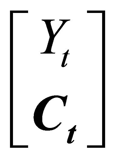
where is an n-vector of quantities of goods consumed in time period t, is an n-vector of quantities of goods consumed in the previous time period, and is the quantity of a composite good at time t representing consumption of all other goods1. We shall assume that the individual consumer maximizes the utility of life-time consumption with utility discounted at rate. With the vector of prices associated with, the consumer’s problem is to maximize

(2)

subject to the intertemporal budget constraint

(3)

where is initial wealth and with initial conditions ².

The first-order conditions (F.O.C.) for utility maximization are

(4a)

(4b)

where is the marginal utility of wealth and is the gradient vector with respect to. Equation (4a), as in [1], is the condition that the marginal utility of the composite good equals the marginal utility of wealth. Equation (4b) generalize the univariate case to the multivariate case where the marginal utility of current consumption of each good plus the discounted value of next period’s marginal utility of consumption equals the marginal utility of wealth times the price of the good. As in [1], the model allows for both harmful addiction

and beneficial addiction

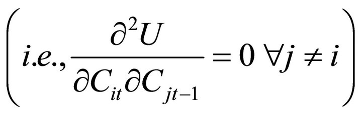
If the consumer takes the marginal utility of wealth constant in formulating decisions for the first-period of his planning horizon, then we can derive marginal utility of wealth constant (Frisch) demand functions showing how current period consumption responds to past, present, and future (expected) prices3. In keeping with a common assumption made when modeling intertermporal demand behavior [4], I assume that the marginal utility of consumption of good i is independent of the quantity of consumption of good j (j ≠ i) of goods consumed in the previous time period

⁴

I also assume that the marginal utility of, while dependent on is independent of⁵.

Assume that the current period utility function can be approximated by a quadratic function so that the F.O.C. can be expressed as⁶

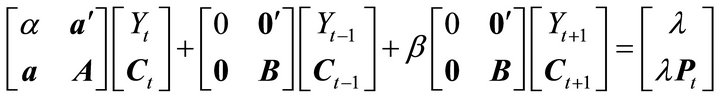(5)

Where

and.

The vector is an n-vector of zeros and is its transpose. The matrix pre-multiplying

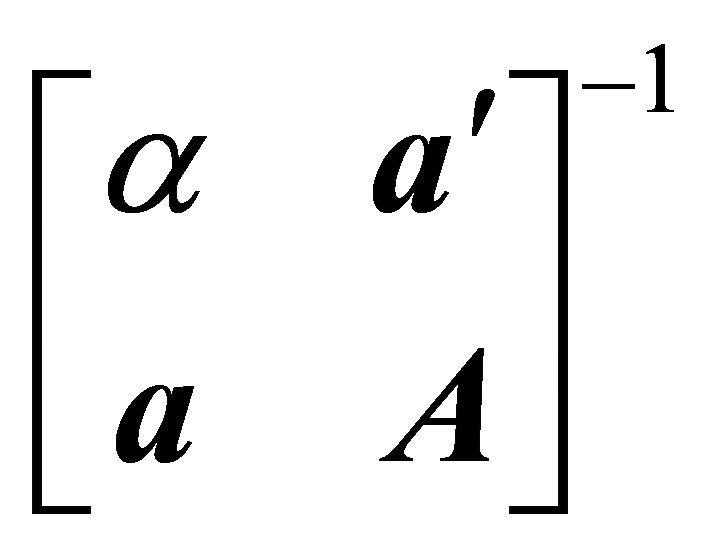
is negative definite. Therefore, its inverse exists and has the following partitioned form:

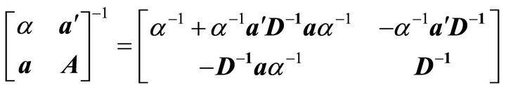(6)

where 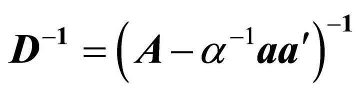is a negative definite matrix, because is the second principal submatrix of

which is negative definite. Given the partitioned inverse (6), the solution to is

(7)

In contrast to the univariate rational addiction model, consumption of good i in the current period is related to lagged consumption of good i, as well as lagged values of all other consumption goods. Moreover, current consumption of good i is related to consumption of all consumption goods in period. Because is negative definite, current period price effects (holding future consumption constant) are negative definite. When is diagonal

3. Stability and General Solution of Matrix Difference Equation

Proposition

When is bounded, the general solution to the matrix difference Equation (7) can be expressed as

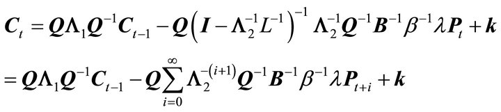
where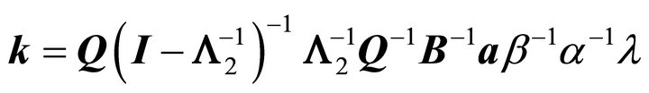, is the diagonal matrix of positive, real eigenvalues which lie within the unit circle, and is the diagonal matrix of positive, real eigenvalues which lie outside the unit circle.

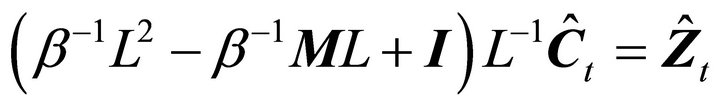
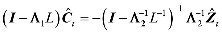
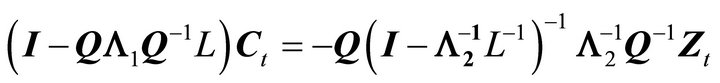
Proof. Rewrite the system of Equation (7) in difference equation form using the lag operator to obtain⁷:

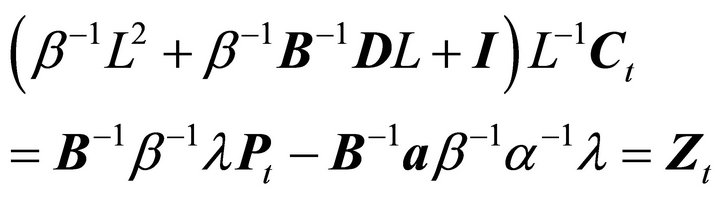(8)

When is a diagonal matrix with positive elements, is positive definite and symmetric because is symmetric negative definite8. Therefore, there exists an orthogonal matrix such that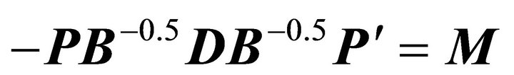, a diagonal matrix with all distinct, positive elements. Define the transformation 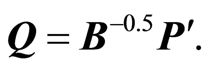Then 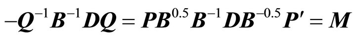. Therefore, and 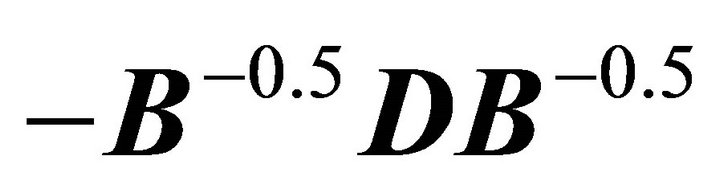are similar matrices [5]. Multiply both sides of (8) by to obtain

or

because. Define and. Then the above equation can be written as

(9)

The matrix polynomial on the left-hand side of (9) can be written as

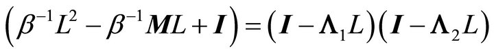(10)

The right-hand side of Equation (10) implies that

(11)

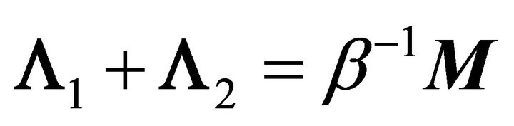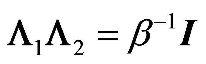where and. The matrix polynomial in (11) is a set of single, second-order difference equations of the form

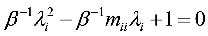
This matrix polynomial consists of individual characteristic equations of the form

. (12)

Because the diagonal elements of are real, we know that 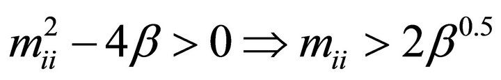and both roots are real and distinct. For stability, 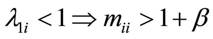and ⁹. By the relationship among roots, 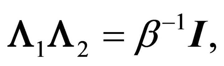this means 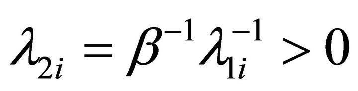when.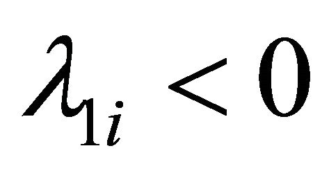

The matrix can be expressed as . Noting also that , the matrix Equation (9) can be written as

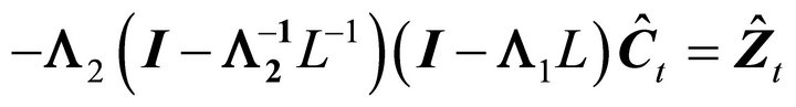(13)

Multiplying both sides by the inverse of yields

Substituting back in terms of and, and multiplying both sides by we obtain

which immediately leads to the desired result.

4. Elasticities

Short-run and long-run elasticities can be derived from the structural parameter estimates. From the above Proposition we see that the price derivatives of the dynamic demand functions are

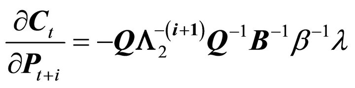(14a)

holding all past prices constant for a temporary price change. For an expected permanent future price change

(14b)

Finally, the long-run price effects are

(14c)

5. An Example

As an example to illustrate the method of calculating the solution to the matrix difference equation and formulas for elasticities consider the two good case which might correspond to two addictive goods such as alcohol and tobacco. Specify the matrices and as follows

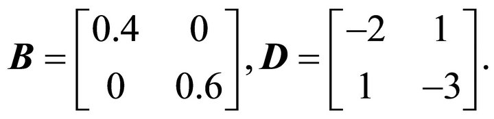
Assuming a discount rate of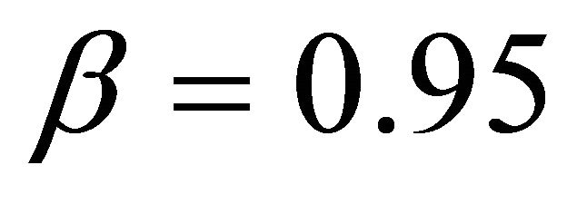, the matrices of eigenvalues associated with are

The matrix consisting of the two eigenvectors associated with the set of eigenvalue is as follows

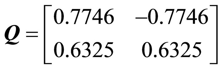
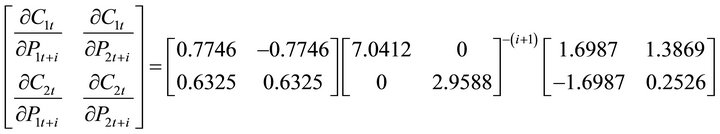
Given these numbers, the solution to the matrix difference equation shown in Proposition is

The matrices of price elasticities shown in Equations (14a)-(14c) are as follows:

(14a’)

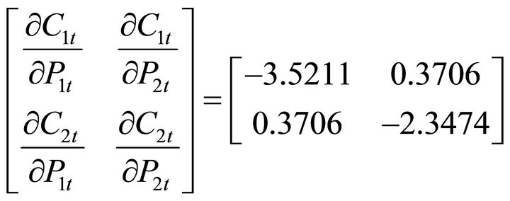(14b’)

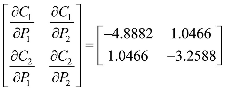(14c’)

This example shows that the solution to the matrix difference equation is stable because the matrix consists of positive real roots all within the unit circle, and the matrix consists of positive real roots all outside the unit circle. The solution also shows that both goods are interrelated in consumption through lagged quantities and current and future prices. Note also that the matrices of price effects as shown in (14a’)-(14c’) indicate that all own-price effects are negative, and all cross-price effects are symmetric and positive. This numerical illustration indicates that we should expect changes in current and future price effects to exhibit complementary effects when both goods exhibit habit formation. In addition, all long-run price effects (in absolute value) should be larger than short-run price effects.

6. Econometric Implications

There is more than one approach to take for quantifying rational addiction behavior. The simplest approach would be to start with the F.O.C. from Equation (5), after eliminating from the set of equations related to, to obtain

(15)

where is a vector of constants, is income, and is a vector of disturbance terms1⁰. The advantage of this specification is that it simplifies imposing and testing for the theoretical restrictions. The testable restrictions are that the matrix, which represents intra-period substitution among the individual consumption goods, is symmetric and negative definite. Thus, the symmetry restriction could be imposed linearly and tested. Because is a matrix of constants, one could also impose negative definiteness on the contemporary substitution matrix using one of the several methods available in the literature (e.g., [7]). The other restriction that one may wish to impose is. With diagonal matrices, this means the restriction is for each equation.

From an econometric point of view, it is straight forward to estimate the model using generalized method of moments by finding instruments such that the orthogonality condition holds, where is a vector of instrumental variables. In this case, as in [1], we could use current, lagged, and futures prices as instruments, in addition to income. If it is not reasonable to assume that consumers know future prices with high probability then we could use current and enough lagged prices sufficient enough to identify the parameters of the F.O.C.

The few attempts to extend the rational addiction model to more than one good ([2], [3]) specify the model as follows

(16)

where is the diagonal matrix whose diagonal elements are so that the ith equation can be written as

(17)

In light of (16), the symmetry constraint, which is now nonlinear, would be imposed as follows:

.

The parameter could then be estimated separately and an estimated value of obtained by dividing the estimate of by.

The other approach to estimation is what [2] and [3] call the reduced-form approach and is indicated by Equation (7), generalized below as follows

(18)

where

This set of equations like (16) has nonlinear restricttions. Equation (18), however, is consistent with the view that the consumer chooses quantities of all goods in the current period simultaneously. It is notable that neither [2] or [3] attempted to utilize these restrictions from theory implied by Equation (16) or Equation (18) in their empirical work.

We typically do not have the luxury to work with panel data at the individual household level. Therefore, it is clear that the estimates of the discount factor may differ from one commodity to another. This is particularly true with aggregate data as in [3], where it is shown that the discount rates for alcohol and tobacco are quite different. To see why estimates based on aggregate data could produce divergent estimates by commodity, note that average consumption of good i, when the discount rate is allowed to be different for each consumer, can be written as follows (over-bars denote simple averages over the total population of consumers):

(19)

where,

is the discount factor for consumer k, is consumption of consumer k for good i at time t+1, and is aggregate consumption of good i. The significant feature of Equation (19) is that the aggregate discount factor is a weighted average of discount factors, each weighted by consumer k’s consumption relative to total consumption. Clearly these weights need not be the same for all consumers. For example, even with the same utility function, a consumer with a higher income could consume a different mix of all consumption goods than a consumer with a lower income. With different discount rates, the average discount rate could be different for different goods. Therefore, for aggregate data, Equation (19) should be modified as follows:

(20)

where is indexed by the particular good consumed. This means different discount rates can be accommodated by the model, while preserving symmetry and negative definiteness in own quantity effects. Note that all the above results still hold when is replaced with, where is the diagonal matrix with diagonal elements 11.

7. Concluding Remarks

This paper formulates and analyzes the multivariate version of the rational addiction model of Becker, Goldman, and Murphy [1]. The multivariate counterpart to the univariate model is that consumption of a specific good in the current period depends on prices of all goods, lagged consumption of all goods, and future consumption of all goods. The theoretical restrictions are that current price effects are negative definite, holding lagged and future consumption constant, and current and past consumption are proportional to one another, the proportionality factor being the consumer’s discount rate. These results indicate that the main restrictions of the univariate model are preserved in the multivariate model.

The conditions in which the model is shown to be dynamically stable are derived. When the model is stable, the solution will have exactly 2n real roots, n of the roots falling within the unit circle and n falling outside the unit circle. The smaller roots can be used to solve the problem backward in time, or to express the current-period solution conditional on the levels of consumption of all goods in the previous period. The set of larger roots are used to express current consumption as a linear function of all future prices. Short-run and Long-run elasticity formulas for the multivariate version are derived and are shown to be generalizations of the univariate version.

Estimation can be undertaken on one of three different forms: 1) The first-order conditions directly, Equation (15); 2) the so-called structural form, Equation (16); or 3) the reduced form, Equation (18). Which of the above approaches to estimation is best can only be determined through further empirical work. Regardless of the approach taken for estimation, the theoretical framework developed in this paper should prove useful to researchers modeling addictive goods that are interrelated in consumption.

8. Acknowledgements

Research supported in part by the North Carolina Agricultural Research Service, Raleigh, North Carolina, 27695.

REFERENCES

NOTES

¹Becker, Grossman, and Murphy [1] also include unobserved lifecycle variables in the utility function. These variables could easily be accommodated in the multivariate version but are not included to simplify the model. For econometric implementations, the main implication is that we would need to assume both lagged and future quantities are endogenous variables because inclusion of lifecycle variables would imply the error term would have a moving average structure.

²Because the price of the composite good is 1, each price of the consumption goods is deflated by the price of the composite good.

³The assumption that λ is constant over the planning horizon is precisely what the model implies. With perfect certainty, the consumer would expect to choose life-time consumption allocations holding λ constant.

⁴In this specification, the effect of a change in lagged consumption of the jth variable on current consumption of the ith good (holding future consumption constant) is, where is the i,jth element of the inverse of the matrix. Thus, current and lagged consumption arestill interdependent when expressed in this form.

⁵This specification generalizes [2] and [3], who also make the marginal utility of independent of.

⁶The quadratic function is not necessary but is introduced in order to evaluate the stability of the system in the neighborhood of the stationary equilibrium. See [1] for a similar approach in the univariate case.

⁷The lag operator is defined as follows: and for any arbitrary vector.

⁸The matrix is the diagonal matrix whose elements are the reciprocals of the square roots of the ‘s. This means then that the matrix is the diagonal matrix whose elements are the square roots of the ‘s.

⁹To see this, note that. If then using (12). So because is decreasing in, in order for [6].

¹⁰We follow [1] in approximating the product of the marginal utility of income and price by a linear function in income and the price. The fixed marginal utility of wealth multiplying price in the linear approximation is then normalized to unity by dividing both sides of the equation by the fixed constant. Since this constant is the same for all equations, the general forms of the matrices in Equation (15) are unchanged.

¹¹Of course, we assume that distribution of effects across individual consumers is relatively constant over time so that can be taken as constant. Otherwise, we would need to modify the model to make a function of variables characterizing changes in the distribution, e.g., proportion of population in different age groups.