Theoretical Economics Letters
Vol. 2 No. 3 (2012) , Article ID: 21516 , 4 pages DOI:10.4236/tel.2012.23052
Rationality and Stability of Equilibrium in a Search-Theoretic Model of Money
Department of Economics, Lehigh University, Bethlehem, USA
Email: tsaito@lehigh.edu
Received May 20, 2012; revised June 23, 2012; accepted July 25, 2012
Keywords: Money-Search; Bargaining Power; Rationality; Stability; Simplification
ABSTRACT
In this short note, I examine the rationality of money-search equilibrium in a basic second-generation money search model, which is a perfectly divisible goods and indivisible money model. I then show that only an inflationary economy can generate a socially and individually rational stable equilibrium. On the basis of this finding, I demonstrate that there is no loss of generality in an analysis that assumes dictatorial buyers in an inflationary economy, since the properties of a dictatorial buyers model are identical to those of a general inflationary economy model. The result of this paper is especially useful for empirical applications since we are generally incapable of finding data showing bargaining power. This result also alerts us against employing the second-generation model to analyze a deflationary economy and commodity money.
1. Introduction
The second-generation money-search model (Trejos and Wright [1]) considers a decentralized market model by using perfectly divisible goods and indivisible money. In the model, each agent judges the goods according to his own taste, and he derives utility from consuming specific goods. Each agent is also endowed with the capability of producing particular product types. Agents live for an infinitely long period and are randomly paired in every period in a Poisson matching process so that the matching process continues forever. In the model, all agents discount the future by a common discount rate represented by β ∈ (0,1). If the paired agents like each other’s products (e.g. double coincidence of wants), they can enter into barter trade. If there is no double coincidence of wants but one likes the product of the paired agent, the one must have “money” to enter into monetary trade.
At the beginning of the entire matching process, money is randomly distributed among agents at probability represented by μ ∈ (0, 1), and it is transferred among them through monetary transactions. Both in barter and monetary transactions, bilateral bargaining determines the quantity of trade (e.g. Nash bargaining solution). The seller in the monetary trade must not be a money holder, as the model does not allow agents to carry more than two units of money. If there is no coincidence, there is no trade. The formal mathematical model is developed as follows.
1.1. Formal Model
Let qd be the quantity of consumption and qs be the quantity of the sale (production) of a particular product type. Given that an agent consumes a product that he likes, we let the utility function be uʹ(qd) for all agents, where uʹ(qd) > 0 and uʺ(qd) < 0. In addition, we let the cost function be c(qs) for all agents for all product types, where cʹ(qs) > 0 and cʺ(qs) ≥ 0. Furthermore, we assume an Inada condition: uʹ(0)  cʹ(0) and uʹ(∞)
  cʹ(∞). The coincidence of wants is supposed to be stochastic, and its probability is given by α ∈ (0,1). The probability of double coincidence of wants is α2 and that of no coincidence is (1 − α)2, so that the probability of single coincidence is calculated as
1 − α2 − (1 − α)2 − α(1 − α) = α(1 − α) (1)
For a seller, once he is paired, the probability of monetary trade is then α(1 − α)μ. Similarly, for a buyer, it is α(1 − α)(1 − μ).
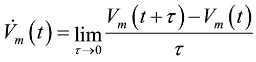
Let V0(t) and V1(t) be the value functions of the nonmoney holder and money holder at period t, respectively, and τ > 0 be the length of each period; hence, the periodical discount rate is approximated by τβ for sufficiently small τ. Let λ0 > 0 be the arrival rate at each moment in the Poisson process. Without loss of generality, we can make τ sufficiently small for λ0 < 1 (e.g., agents are paired once per period at most). Let p0 = α(1 − α)μλ0 be the probability for a buyer meeting a seller to make a monetary transaction in the matching process and p1 = α(1 − α)(1 − μ)λ0 be that of a seller meeting a buyer to make a monetary transaction. Let p2 = α2λ0 be the probability of barter trade between both the buyer and seller. In this specification, τpm represents the probability of each event m ∈ {0, 1, 2} per period. Let  be the time derivative of Vm(t) so that
 (2)
(2)
Then, for τ → 0, the Bellman equation for the seller satisfies
 (3)
(3)
where 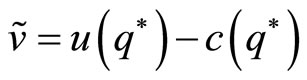 is the net utility from barter trade and
 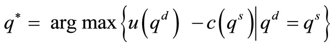 is the instantaneous social welfare maximizer (Appendix 1). Similarly, the Bellman equation for buyer satisfies
 (4)
(4)
where γ is the constant utility flow to store a unit of money for a period; hence γ < 0 implies that money is costly to store (fiat money) and vice versa for γ > 0 (commodity money).
1.2. Search Equilibrium
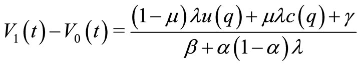
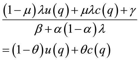
In the equilibrium, we have qd = qs = q, since demand and supply must be equal, where q is given as a Nash bargaining solution (Appendix 2) that satisfies V1(t) − V0(t) = (1 − θ)u(q) + θc(q) (5)
where θ ∈ [0, 1] represents the bargaining power of the buyer in the Nash product. The two Bellman equations are then solved as
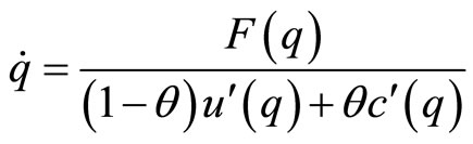 (6)
(6)
In Equation (6), F(q) is given by
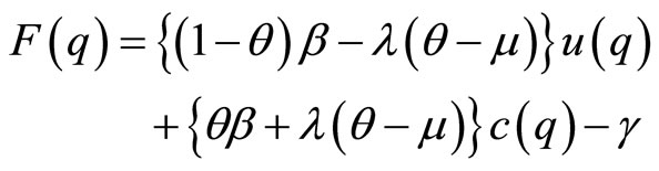 (7)
(7)
where λ = α(1 − α)λ0 is the arrival rate of a single coincidence.
Remark 1. F(q) is  -shaped in q iff μ < θ and λ > (θ − μ)−1(1 − θ)β; ∩-shaped in q iff μ > θ and λ > (θ − μ)−1θβ; and otherwise monotonically increasing in q.
Proof. By differentiating F(q), we find that
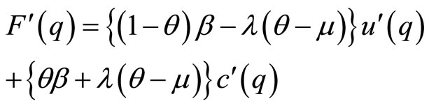 (8)
(8)
Since utility and cost functions are monotonically increasing in q, we can say that F(q) is ∪-shaped if and only if F ʹ(0) < 0 and F ʹ(∞) > 0; it is ∩-shaped if and only if F ʹ(0) > 0 and F ʹ(∞) < 0, monotonically increasing if and only if F ʹ(0) > 0 and F ʹ(∞) > 0, and monotonically decreasing if and only if F ʹ(0) < 0 and F ʹ(∞) < 0. Since uʹ(0) ≫ cʹ(0) and uʹ(∞) ≪ cʹ(∞), the sign of F ʹ(q) at q = 0 is identical to the coefficient of uʹ(0) and at q → ∞ to that of cʹ(∞) in Equation (8). By rearranging the terms of (1 − θ)β – λ(θ − μ) ⋛ 0 for q = 0 and θβ + λ(θ − μ) ⋛ 0 for q → ∞, we obtain the conditions for each shape of F(q) as stated in this remark. We then find that the two inequalities do not satisfy the condition for the monotonically decreasing case.
Q.E.D.
The classification of F(q) stated in Remark 1 is depicted in Figure 1. As is shown in this figure, F(q) cannot be ∪-shaped if θ ≤ μ, and it cannot be ∩-shaped if θ ≥ μ. For later use in the final remark, we remark as follows.
Remark 2. If θ = 1, as a dictatorial buyers model, F(q) cannot be ∩-shaped.
Since (1 − θ)uʹ(q) + θcʹ(q) > 0,  ⋛ 0 is equivalent to F ʹ(0) ⋛ 0; hence, the equilibria are given by F(q) = 0, as depicted in Figure 2. Note that we cannot have stable equilibrium in the ∪-shaped case if γ > 0 since the intercept is −γ. An equilibrium is stable if and only if we have F ʹ(q) < 0 (cross the horizontal axis from above). We can then find that a shift of F(q) toward the same direction creates opposite comparative statical results for the stable equilibria in the ∪-shaped F(q) and ∩-shaped F(q). For example, an increase in μ creates an upward shift of F(q) if the monetary trade is socially rational: u(q) ≥ c(q). In such a case, we conclude that the price level 1/q increases in the ∩-shaped case, while it declines in the ∩-shaped case. Therefore, it is very important to identify which shape appears in the analysis, unless we do not consider the rationality conditions, as in the next section.
2. Rationality and Stability of Equilibrium
Using Equations (3) and (4), we consider V1(t) − V0(q) at the steady state 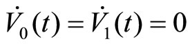 to get
 (9)
(9)
At the equilibrium, the above value, Equation (9) is equal to the value that is given by the Nash bargaining solution, Equation (5); whence, we find
 (10)
(10)
This equation is further arranged as

Figure 1. Classification of F(q) in terms of μ and θ.

Figure 2. Examples of stable and unstable equilibria for each F(q).
 (11)
(11)
Therefore, if money is costly to store as fiat money in an inflationary economy (γ ≤ 0), u(q) ≥ c(q) holds if and only if θβ + λ(θ − μ) > 0, that implies that F(q) is a ∪-shaped function (Remark 1).
Proposition 1. In an inflationary economy, F(q) is ∪-shaped so long as the monetary transaction is socially rational.
Next, we consider money that is not costly to store as commodity money or as fiat money in a deflationary economy (γ > 0). In this case, to obtain stable equilibrium, F(q) must be ∩-shaped, so that θβ + λ(θ − μ) < 0. Then, for social rationality u(q) ≥ c(q), from Equation (11), we must have
βu(q) ≤ γ. (12)
For a money holder, participation in the matching market is individually rational if and only if a transaction is better than storing money forever, so that we must have
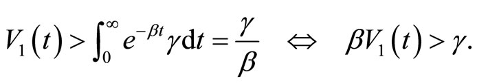 (13)
(13)
From Equations (12) and (13), we find that V1(q) > u(q). (14)
However, Equation (14) implies that holding money is better than using money to obtain instantaneous utility; hence, no trade occurs.
Proposition 2. A commodity money economy or fiat money deflationary economy cannot generate socially and individually rational stable monetary equilibrium.
3. Final Remarks
This note has shown that stable equilibrium cannot be obtained if γ > 0 (Proposition 2). If γ ≤ 0, we can obtain a stable equilibrium and F(q) is ∪-shaped (Proposition 1). The two results imply that we can assume a dictatorial buyer (θ = 1) without loss of generality so long as we focus on the stable monetary trade equilibrium (Remark 2). This result is especially useful for empirical applications (for example, Saito [2]) since we are generally incapable of finding data showing bargaining power. Yet, it should be noted that the result in welfare analysis would be affected by the choice of bargaining power and bargaining mechanism as suggested by Aruoba et al. [3]. At the same time, the result in this paper also suggests that we cannot analyze commodity money and a deflationary economy in this framework if we care about the stability of equilibrium.
4. Acknowledgements
This article is based on a part of my Ph.D. dissertation submitted to the State University of New York at Buffalo [2]. I am truly grateful to Professors Winston Chang and Peter Morgan for several helpful comments and encouragements. I also wish to thank the editor and an anonymous referee. All possible remaining errors and shortcomings are still mine.
REFERENCES
- A. Trejos and R. Wright, “Search, Bargaining, Money, and Prices,” Journal of Political Economy, Vol. 103, No. 1, 1995, pp. 118-141. doi:10.1086/261978
- T. Saito, “Toward a Search-Theoretic Approach of Modern Economic Growth, Financial Deepening, and Urbanization: A Cross-Country Perspective,” Ph.D. Dissertation, State University of New York, Buffalo, 2011, pp. 3-50.
- S. B. Aruoba, G. Rocheteau and C. Waller, “Bargaining and the Value of Money,” Journal of Monetary Economics, Vol. 54, No. 8, 2007, pp. 2637-2655. doi:10.1016/j.jmoneco.2007.07.003
- H. M. Ennis, “On Random Matching, Monetary Equilibria, and Sunspots,” Macroeconomic Dynamics, Vol. 5, No. 1, 2001, pp. 132-142. doi:10.1017/S1365100501018065
Appendix 1. Nash Bargaining Solution in Barter Trade
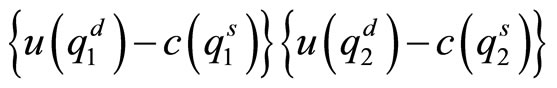
Let i = 1, 2 be the index of an individual agent in a barter-trade pair to denote  and
and  as demand and supply of the individual i. Let us assume equal bargaiing power between the two agents. Since there is no transfer of money in barter trade, its Nash bargaining solution is given by maximizing
 (15)
(15)
The market clearing conditions require 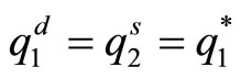 and
and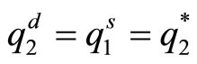 . Substituting the conditions to maximize with respect to
  and
and  and rearranging the terms provide the first order condition as
 (16)
(16)
If  is socially optimum, it satisfies the first order condition, as
 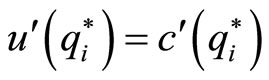 and
and . If it is not a social optimum, it cannot satisfy the first order condition consistently with the equal bargaining power assumption. Therefore, the quantity of trade in barter trade is the social optimum.
Appendix 2. Nash Bargaining Solution in Monetary Trade
Let 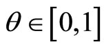 be bargaining power of the buyer (measured in an increasing manner). Then, the Nash bargaining solution for monetary trade is given by
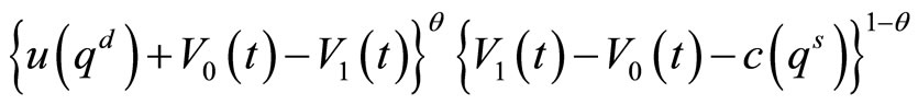 (17)
(17)
In accordance with the splitting rule based on θ (see also Ennis [4]), we find that the solution qd = qs = q* satisfies the splitting rule (Nash bargaining solution) such that
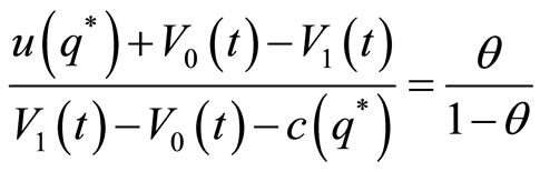 (18)
(18)
which is further rearranged to obtain Equation (5). Subsequently, we can also find that
 (19)
(19)
This equation is applied to obtain the law of motion function, as Equation (6).