ABSTRACT

Abundant evidence indicates that financial asset returns are thicker-tailed than a normal distribution would suggest. The most negative outcomes which carry the potential to wreak financial disaster also tend to be the most rare and may fall outside the scope of empirical observation. The difficulty of modelling these rare but extreme events has been greatly reduced by recent advances in extreme value theory (EVT). The tail shape parameter and the extremal index are the fundamental parameters governing the extreme behavior of the distribution, and the effectiveness of EVT in forecasting depends upon their reliable, accurate estimation. This study provides a comprehensive analysis of the performance of estimators of both key parameters. Five tail shape estimators are examined within a Monte Carlo setting along the dimensions of bias, variability, and probability prediction performance. Five estimators of the extremal index are also examined using Monte Carlo simulation. A recommended best estimator is selected in each case and applied within a Value at Risk context to the Wilshire 5000 index to illustrate its usefulness for risk measurement.

Keywords:

Tail Risk, Extreme Value Theory, Clusters, Value at Risk, Expected Shortfall

1. Introduction

Abundant evidence, dating back to early work by Mandelbrot [1] and Fama [2] , indicates that financial asset returns are thicker-tailed than a normal distribution would suggest. The most negative outcomes, which carry the potential to wreak financial disaster, also tend to be the most rare and sometimes fall outside the scope of our empirical observation. Understanding these “tail risks” has been at the heart of the recent push for better risk measurement and risk management systems. This includes efforts under the 2010 Dodd-Frank Act to better identify sources of systemic risk as well as academic work aimed at pricing tail risk (Kelly and Jiang ( [3] [4] ). Value at risk (VaR) and the related concept of expected shortfall (ES) have been the primary tools for measuring risk exposure in the financial services industry for over two decades, yet when these measures rely upon empirical frequencies of rare events, they tend to underestimate the likelihood of very rare outcomes.

More recently, the difficulty of modelling rare but extreme events has been greatly reduced by advances in extreme value theory¹. From this body of research, two parameters have been found to play a central role in the modelling of extremes: the tail shape parameter ξ and the extremal index θ. In brief, let (Y_T) be a sequence of i.i.d. random variables with distribution F and M_T = max(Y₁, …, Y_T). It can be shown that as T ? ∞, a suitably normalized function of M_T converges to a non-degenerate distribution function G(Y; ξ), and if (Y_T) is a strictly stationary time series, then it converges to G(Y; ξ, θ). The tail shape parameter describes how quickly the tail of the return distribution thins out and governs the extreme behavior of the distribution. The extremal index describes the tendency of extreme observations to cluster together, a common feature in data series showing serial dependence.

This study examines, within a Monte Carlo context, five estimators for the tail shape parameter and five estimators for the extremal index that have been proposed in the literature. While there have been various isolated studies of the properties of some of these estimators, there does not appear to be a comprehensive study of the properties of all of these estimators found anywhere in the literature². The purpose of this study is twofold. From an academic viewpoint, I address the question of which estimators show more desirable properties, especially their finite sample behavior using typical financial dataset sizes. From a practical viewpoint, I address the question of which estimator a practitioner should choose from among a number of available options proposed in the literature. In other words, “Does any particular estimator for the tail shape or for the extremal index stand out above the alternatives?” In addition to providing evidence on the finite sample performance of the estimators, a specific recommendation is made for a “best” overall choice in each case. An application of the preferred estimators to Wilshire 5000 index returns is also given to demonstrate the usefulness for risk management purposes.

Estimation of the tail shape parameter is first introduced using a collection of relative maxima from sub-intervals of the data sample. This early approach to estimating the tail shape is known as the “block maxima” method and is provided for historical context and to contrast with the more recent estimators that are the focus of this study. The tail shape parameter is then estimated using the peaks over threshold (POT) approach, a more efficient method which uses all observations for estimation that exceed an arbitrary quantile of the data. Under this approach a quantile of the distribution is chosen (for example the 95^th quantile) and all observations that exceed this are considered extreme and used for estimation of the tail shape parameter. Five tail shape estimators based on the POT approach that have been proposed in the literature are introduced. Each of the five tail shape estimators is assessed through Monte Carlo simulation along the dimensions of bias, root mean squared error, and overall stability across a range of distributional thresholds.

The extremal index measures the tendency for observations in the extreme tails of the distribution to cluster together. Four of the five estimators for the extremal index require that the data be partitioned into sub-intervals, called “blocks”, in order to look for clustering. I analyze the tradeoff between data independence and availability in selecting block size. The goal in choosing a block size is to select an interval long enough that, even though there may be clustering within the blocks, the blocks themselves are, in effect, independent of one another. For the extremal index, each estimator is assessed along the dimensions of bias, root mean squared error, and overall stability across a range of distributional thresholds.

This study gives an overall recommendation for the best tail shape estimator, including the data threshold at which it tends to work best, and a proposed bias adjustment. I also give an overall recommendation for the best extremal index estimator, including the data threshold at which it tends to work best. The results also shed light on which estimators are useless from a practical standpoint. The best estimator from each category is used to highlight the usefulness of these tools in risk management applications. These results are not only of academic interest, but are of potential interest to practitioners, who rely upon estimated risk parameters as inputs to their risk forecasting models.

2. Overview of Extreme Value Theory

Extreme value theory (EVT) is an approach to estimating the tails of a distribution, which is where rare or “extreme” outcomes are found. This branch of statistics originally developed to address problems in hydrology, such as the necessary height to build a dam in order to guard against a 100-year flood, and has since found applications in insurance and risk management. For financial institutions, rare but extremely large losses are of particular concern as they can prove fatal to the firm. In 1995 the Basel Committee on Bank Supervision, a committee of the world’s bank regulators that meets periodically in Basel, Switzerland, adopted Value at Risk (VaR) as the preferred risk measure for bank trading portfolios. VaR, which is simply a quantile of a probability distribution, is very intuitive as a risk measure and has since become a popular standard for risk measurement throughout the financial industry. In practical risk management applications, forecasting relies upon historical data for estimation of future outcomes. However, extreme rare events are, by nature, infrequently observed in empirical distributions. EVT can be used to improve probability estimates of very rare events or to estimate VaR with a high confidence level by smoothing and extrapolating the tails of an empirical distribution, even beyond the limits of available observed outcomes in the empirical distribution.

Classic statistics focuses on the average behavior of a stochastic process, and a fundamental result governing sums of random variables is the Central Limit Theorem. When dealing with extremes, the fundamental theorem is the Fisher-Tippett Theorem [9] , which gives the limit law for the maxima of i.i.d. random variables³. Suppose we have an i.i.d. random variable Y with distribution function F, and let G be the limiting distribution of the sample maximum M_T. The Fisher-Tippet Theorem says that under some regularity conditions for the tail of F and for some suitable constants a_T and b_T, as the sample size T ? ∞,

(1)

where G(y) must take the following form:

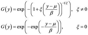(2)

which is the Generalized Extreme Value (GEV) distribution. It has three parameters: location (μ), scale (β), and shape (ξ). The shape parameter ξ governs the tail behavior, giving the thickness of the tail and plays a central role in extreme value theory. The GEV distribution encompasses a wide range of distributions that fall into three main families, depending upon the value of ξ:

Type I: Gumbel ξ = 0, “thin tailed”.

Type II: Fréchet ξ > 0, “fat tailed”.

Type III: Weibull ξ < 0, “short tailed”.

Thin-tailed (ξ = 0) distributions exhibit exponential decay in the tails and include the normal, exponential, gamma, and lognormal. Short-tailed (ξ < 0) distributions include the uniform and beta and have a finite upper end point. Heavy-tailed distributions (ξ > 0), which fall under the Fréchet, are of particular interest in finance, and include the Student-t and Pareto.

Financial returns are known to have thick tails compared to a normal distribution, and a number of alternative distributions have been posited to capture this feature of the data, with varying success. However, for modelling extremes we do not need to dwell on the entire distribution since large losses are to be found in the tails. Thus, the central result of EVT theory, that the tails of all distributions fall into one of three categories, greatly simplifies the task of the risk analyst. The only remaining obstacle is to estimate, as accurately as possible, the shape parameter ξ from the data. Value-at-risk formulas that incorporate the tail shape parameter, as well as standard probability functions, may then be applied to measure risk.

While the Fisher-Tippett Theorem says that maxima are GEV distributed, in order to be useful for estimation purposes, we need more than just one sample maximum (i.e. one observation) from which to estimate the three distributional parameters. In order to generate more observations, we may divide a sample into many sub-samples, or “blocks”, and compute the local maximum from each block. A block would need to be large enough to give fairly rare, or extreme, observations for maxima. For example, taking the maximum daily return out of weekly blocks (1 of every 5 observations) would encompass 20% of the distribution and likely fail to capture only extreme values. Local maxima drawn from monthly blocks (1 of every 21 daily returns) may still be insufficient to focus on the most extreme values. Increasing the block size to quarterly, for example, will serve to produce more extreme maxima, but will also decrease the number of useable observations. Thus, when attempting to estimate parameters of the GEV distribution by the blocks method, one faces a fundamental tradeoff between choosing more, but less extreme, observations, or fewer observations that are relatively more extreme.

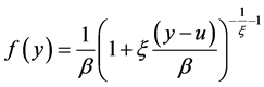
Since thick-tailed distributions are of particular interest, and ξ = 0 corresponds to distributions that are thin-tailed, we focus on the case ξ ≠ 0. Differentiating G(y), we get the pdf of the GEV:

(3)

Taking logarithms and summing, we get the log likelihood function:

(4)

As an example of how the GEV distribution may be used to estimate the tail shape parameter, we consider daily logarithmic returns data for the Wilshire 5000 stock index over January 1, 1996, through December 31, 2015. Figure 1 displays the data, which shows episodes of increased volatility and relatively extreme returns. Suppose the data are partitioned into localized blocks according to calendar month, with each block having approximately 21 returns. Panel A of Figure 2 shows the maximum (negative) return within each monthly block. Note that the observations are not necessarily equally spaced because the most extreme observation may have occurred at any time during the block. If the data are instead partitioned into localized blocks according to calendar quarter, this results in each block having approximately 63 returns. Panel B of Figure 2 shows the maximum (negative) return within each quarterly block. The quarterly blocks are larger, fewer in number, and are clearly capturing the more extreme returns compared to the monthly blocks.

The tail shape parameter ξ is estimated by maximum likelihood under the GEV distribution in Equation (4) for both the monthly and then quarterly block maxima and results are presented in Table 1. The tail shape estimate from the monthly block maxima is ξ = 0.181 with a t-statistic of 3.63, indicating significantly fatter tails than the normal distribution. The tail shape estimate based on the quarterly block maxima, however, is almost double at ξ = 0.330 with a t-statistic of 2.51. While both estimates agree that the underlying stock return distribution is fat-tailed, these estimates show some disparity in the degree of extreme behavior, depending upon the choice of block size.

The block maxima approach to estimating tail shape only keeps one observation from each block, which is wasteful of data and requires a large sample for accurate parameter estimation. A more recent and popular approach to estimating tail shape selects a quantile of the distribution as a threshold, above which all data are treated as extreme and used for estimation. This approach is known as the Peaks over Threshold (POT) method, and makes more efficient use of the data because it uses all large observations and not just block maxima. The POT approach depends on a theorem due to Pickands [11] and Balkema anddeHaan [12] , which says that the limiting distribution of values above some high threshold u of the data is a Generalized Pareto Distribution (GPD):

(5)

Panel A: Monthly Block Maxima

The GPD is very similar to the GEV and is governed by the same tail shape parameter ξ. The distribution is heavy-tailed when ξ > 0, becoming the Fréchet-type. If ξ = 0 it becomes the thin-tailed Gumbel-type, which includes the normal, and if ξ < 0 it is of the short-tailed Weibull-type. This says that not just the maxima, but the extreme tails themselves, obey a particular distribution and are governed by the same tail shape parameter ξ as in the GEV. The Fréchet class of heavy-tailed distributions remains the focus of interest in financial applications and in this study. It is useful to note that the mth moment of Y, E(Y^m), is infinite for m ≥ 1/ξ.

3. Tail Shape Estimators

Tail shape estimators based on the POT approach fall under the semi-parametric and fully parametric type. I next introduce five estimators for the tail shape ξ that have been proposed in the literature. The first is fully parametric based directly on the GPD and the principle of maximum likelihood. The other four estimators are semi-parametric, since they do not assume a distributional form for estimation purposes.

Define:

y = data sample.

T = sample size.

q = quantile of the distribution (e.g. q = 0.99).

u = data threshold corresponding to quantile q.

n = number of exceedances over threshold u.

ξ = tail shape parameter.

β = scale parameter.

Denote the order statistics of the sample as y₍₁₎ ≤ y₍₂₎ ≤ …≤ y_(T).

3.1. Maximum Likelihood Estimators

A fully parametric estimator of ξ may be obtained by taking the derivative of the generalized Pareto distribution function in Equation (5) and applying maximum likelihood techniques. The derivative of Equation (5) is the pdf of the GPD with parameters ξ and β:

(6)

and the log-likelihood function is

(7)

with solutions and satisfying:

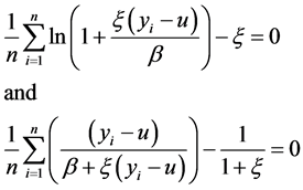(8)

The maximum likelihood estimator is valid for values of ξ > −1/2, and an estimate of the scale parameter β, which is useful for VaR calculations, is also obtained by this method.

3.2. Hill Estimator

The semi-parametric estimator proposed by Hill [13] is valid for ξ > 0 and is simple to compute from the n upper order statistics of the sample above a given threshold u.

(9)

3.3. Pickands Estimator

The semi-parametric estimator proposed by Pickands [11] is valid for ξ Î ℝ and brings in information further toward the center of the distribution. For example, if the chosen threshold defining extreme data is the 5% tail, the Pickands estimator would also look at the order statistics at the 10% and 20% quantiles.

(10)

3.4. Dekkers-Einmahl-de Haan Estimators

The estimator proposed by Dekkers, Einmahl, and de Haan [14] seeks to improve upon the original Hill estimator by bringing in a second-order term. This estimator also has the benefit of being valid over the entire real numbers, ξ Î ℝ, rather than for positive values of ξ only. Thus, it should be able to detect tails in all three classes, not only the Fréchet class of distributions. In addition to an estimator for tail shape, the authors propose an estimator for the scale parameter, β.

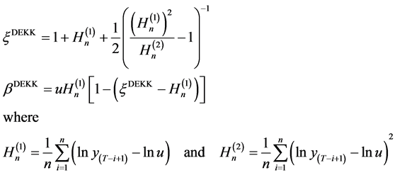(11)

Note that is simply the Hill estimator.

3.5. Probability-Weighted Moment Estimators

The Probability-Weighted Moment (PWM) estimator was proposed by Hosking and Wallis [15] and is valid for ξ < 1. This estimator assigns weights to the extreme order statistics, with more extreme values receiving smaller weight. By using a weighting scheme, this approach seems intuitive, but relies more on values that are closer to the center of the distribution than do other estimators such as the Hill estimator.

(12)

4. Monte Carlo Analysis of Tail Shape Estimators

For the Monte Carlo study, I initially set the sample size at T = 2000 observations. This would roughly correspond to eight years of daily financial returns data, assuming 252 trading days in a year. Data are randomly generated from a Student-t distribution with v degrees of freedom in order to make use of the convenient fact that the tail shape parameter ξ for a Student-t distribution is known to equal 1/v.

In order to implement peaks over threshold (POT) estimation, there yet remains the issue of needing to choose a threshold of the distribution over which all data are to be treated as extreme. If we set a relatively low boundary, for example the 90^th percentile, and work with the upper 10% of order statistics in the distribution, we risk including data that are not really that extreme and for which the underlying extreme value theory is less likely to hold. This can lead to an inaccurate, biased estimate. On the other hand, suppose we choose a very high threshold of the data, such as the 99^th percentile, and use just the extreme upper 1% for estimation. Given the finite size of empirical datasets, we are likely forced to base our inference on a small number of observations, leading to very noisy estimates. A common rule of thumb in applied work sets a threshold of at least the 95^th percentile as a cutoff to define the extreme tail. To illustrate the potential tradeoffs across a range of distributional cutoffs, I conduct a Monte Carlo simulation of 200 trials of T = 2000 observations from a Student-t distribution with 4 degrees of freedom. This produces a tail shape value of ξ = 0.25, and is similar to many financial data series, which often fall in the range 0.20 to 0.35. For each simulation trial, I estimate ξ using data above quantile q, where q is sequentially varied over the range q = 0.9500 to q = 0.9975 in increments of .0025. For each quantile cutoff q, I estimate ξ using each of the five estimators: ML, Hill, Pickands, Dekkers, and PWM.

The average results from 200 simulation trials are reported in Table 2 and, for ease of

comparison, displayed in Panel A of Figure 3. First, note that all of the estimators show some degree of bias for almost every choice of q, with no estimator consistently achieving the correct value of ξ. For a sample of 2000 observations, a threshold at the 95^th percentile leaves 100 observations for estimation, whereas a cutoff at the 99^th percentile leaves only 20 data points for estimation. Thus, as we move to the right along the x axis, the estimators are expected to become somewhat less precise and more variable, particularly in the very high quantiles. The Hill estimator displays a large upward bias at q = 0.95, and this gradually declines as q ? 1. The Dekkers estimator is slightly downward biased at q = 0.95 and remains remarkably stable as q ? 1. The Pickands estimator has an enormous downward bias at q = 0.95 and only begins to approach the accuracy of other estimators as q ? 1, while becoming noticeably less stable. The probability- weighted moments estimator performs similarly to Dekkers for q = 0.95, with a downward bias, but becomes unbiased and then unstable as q ? 1. The ML estimator shows more downward bias than either Dekkers or PWM, and it becomes very unstable as q ? 1.

Panel B of Figure 3 displays results for the case of ξ = 0.50, which is at the upper boundary of interest for many finance applications, as values beyond this point are rare and imply that the distribution lacks a finite second moment. The same patterns seen in Panel A are generally present in this case. However, the Hill estimator performs noticeably better, showing less bias. Panel C shows results for an important special case―

namely, that of no fat tails. The data for the simulation in Panel C was generated from a normal distribution, which has ξ = 0. This is an important case to examine, because a good estimator should not give a false positive by indicating the presence of a fat tail when there is none. We see that the Hill estimator stumbles badly here. At the threshold of q = 0.95, which is commonly adopted for empirical work, the Hill estimator reports a fat tail of ξ = 0.21 when in fact the distribution is thin-tailed. The other four estimators are downward biased, giving slightly negative values for the tail shape. Of these, Dekkers and ML are the most stable, changing little over the range q = 0.95 to q = 0.99.

The results discussed so far are based on a generous sample size of 2000 observations. However, the empiricist is quite often faced with a more limited amount of data from which to draw conclusions. Therefore, I next repeat the above analysis using a sample size of T = 500 observations. At a quantile cutoff of q = 0.95, for example, this would leave only 25 observations in the tail for extreme inference. How do the estimators perform when given so few observations to work with? The tradeoff between bias and variance becomes much more apparent under these circumstances when looking at Figure 4. Focusing on Panel A, which shows the case of ξ = 0.25, Dekkers appears to be the most stable estimator across different choices of threshold q. Although not highly unstable, Hill exhibits substantial variability across quantiles, with its value depending on the quantile q that is chosen. For low quantile cutoffs, Hill is positively biased, and this bias disappears and then becomes negative as q ? 1. PWM is unbiased at lower quantiles, but becomes highly unstable above the 97^th quantile. Both Pickands and ML are extremely negatively biased and unstable.

Panel B shows results for ξ = 0.50. All of the patterns observed for ξ = 0.25 in Panel A reappear here, except that Deckers now shows more of a downward bias and some decline in value as q ? 1. The Hill estimator seems unbiased for low values of q, but exhibits a greater decline in value as q ? 1. In Panel C, we examine the important case of a thin tail where ξ = 0, now with the added complication of a small sample size. The two most accurate estimators, for smaller q values, are Dekkers and PWM. However, we see again that PWM is unstable. As q ? 1 and the amount of extreme tail data used for estimation drops, PWM becomes highly biased and variable. Dekkers, however, continues to be relatively stable and accurate as q ? 1. ML and Pickands are extremely negatively biased and unstable. Hill is again seen to give a false positive, with its large positive bias indicating a fat tail when none exists. The magnitude of this bias declines as q ? 1.

Overall, we may draw the following conclusions. The Pickands and ML estimators are extremely biased for any q less than about 0.99, but become very unstable as q moves above 0.97. The Hill estimator is upward biased, becoming more so as ξ falls below 0.50, and is unable to detect thin tails, reporting positive ξ when none exists⁴. The

PWM estimator performs well at a quantile value of q = 0.95, generally with a downward bias. This bias is directly dependent on the size of the dataset, while holding q fixed at the 95^th percentile, a behavior also exhibited by the ML estimator. The bias of the PWM estimator at q = 0.95 shrinks almost to zero for the smaller dataset of T = 500 observations. Because of the shifting bias of the PWM estimator, I conclude that the best all-around estimator is the Dekkers estimator, which is slightly downward biased⁵. This estimator is quite stable for quantile values of q from 0.95 to 0.99, performing best around q = 0.95. This is a substantial advantage when dealing with smaller datasets, where Pickands and ML, which require a higher data threshold, become useless.

5. Risk Management Applications

5.1. Value at Risk

One of the primary applications of interest for tail measurement is in the area of financial risk management and the calculation of value-at-risk (VaR)⁶. The VaR statistic may be defined as the worst expected loss with a given level of confidence Q, and is simply a quantile of the payoff distribution. For a desired quantile Q (e.g. for a 99% VaR, Q = 0.99) the VaR statistic may be derived from the GPD distribution:

(13)

A related concept is the “T level.” This is the data value which is expected to be exceeded once, on average, every T periods. To find the T level, we set (1 ? Q) in the VaR formula equal to the event frequency of interest. To find the T level for the entire sample of size T, set (1 ? Q) equal to 1/T:

(14)

For example, if the entire data sample of size T is comprised of 1008 daily observations (4 years of daily returns data) and one wishes to find the return level that is expected to be exceeded once every four years, on average, (the “4-year level”), then set (1 ? Q) = 1/1008. The probability of exceeding any arbitrary threshold x above u may also be derived from the GPD distribution:

(15)

We see that for VaR and related calculations, it is necessary to also obtain an estimate of the scale parameter β. We have three choices for estimating β : maximum likelihood, Dekkers, and probability-weighted moment. Accurate estimation of β is essential in order to obtain accurate inference on extreme values in the tail, such as computing the T-level and related probabilities. In essence, estimation of the parameter β calibrates the theoretical tail shape to the empirical tail of the distribution and tends to work best for EVT purposes when estimated at a very high quantile of the data. It is important to stress that β is thus not necessarily estimated at the same quantile of the distribution at which ξ is estimated, and it is in fact usually not optimal to do so. By “calibrating” the theoretical tail to the empirical tail of the distribution at a very high quantile of the data, such as q = 0.995, we are better-positioned to obtain accurate probability estimates of extreme outcomes.

5.2. T-Level Exceedance Predictions

I propose to use the T-level as an accuracy benchmark for the pair of EVT parameters in the following manner. For a simulated Student-t dataset of length T = 2000 observations, I estimate ξ at a quantile cutoff of q = 0.95 using Dekkers, ML, and PWM, and I estimate β by each method at a cutoff of q = 0.995. For the maximum likelihood method, this involves concentrating out the tail parameter ξ by feeding the value estimated by ML at q = 0.95 into the second likelihood function as a fixed value when estimating β. With each of three sets of parameters (ξ, β), I estimate three T-levels using Equation (14) and check how many times (if at all) each T-level was actually exceeded in the simulated data. Recall that the T-level should be exceeded once in expectation, though this may or may not occur in any one realization of a data sample. However, over a large number of simulations, the T-level should be exceeded once on average for an accurate estimator. Viewing 2000 simulated observations as daily financial returns would give 2000/252 = 7.94 years of daily data, so I also compute the 1-year level. This is the level that should be exceeded once a year, or 7.94 times in a sample of this size.

I run 1000 simulation trials and report the results in Table 3. Panel A shows the frequency in which the T-level was exceeded for each set of estimators over the 1000 trials. The PWM estimators clearly perform the worst out of the three, with 1.61 exceedances on average. This implies that PWM tends to set the T-level too low and it is easily exceeded in sample. Dekkers is the closest to the ideal number of one exceedance on average, with a mean of 1.05, though the ML estimators are surprisingly close at 1.07. This is surprising due to the larger bias exhibited by the ML estimates of ξ compared to Dekkers observed earlier. When paired with a beta estimated through maximum likelihood, the set of ML estimators manages to still give reasonably accurate probability estimates. Panel B tabulates results for the 1-year level, which is the level expected to be exceeded 7.94 times in a dataset of 2000 observations. This level is smaller, or less extreme, than the full-sample T-level, and constructs another test for the ability of these estimators to provide useful information to the risk analyst. The PWM estimators show an average of 8.29 exceedances, compared to 7.77 for ML and 7.81 for Dekkers. Maximum

likelihood and Dekkers are again close to each other and fairly close to the expected number of 7.94 exceedances.

5.3. Application to the Wilshire 5000 Index

Based on results for parameter bias, root mean squared error, stability across quantiles, and T-level accuracy, I believe that the Dekkers estimator is a preferable choice over the alternatives. Accordingly, as a real-world application of these risk management tools, I use the Dekkers estimators on the Wilshire 5000 data in order to compute some VaR- based statistics. The Dekkers-based estimate of the shape of the left tail of the Wilshire returns distribution is ξ = 0.282. To gauge the precision of the estimate, I implement a bootstrap procedure that resamples the Wilshire data with replacement and re-esti- mates ξ each time in order to generate a standard error. Based on 200 bootstrap samples, this gives a t-statistic equal to 4.35 for ξ, indicating that the Wilshire 5000 is significantly fat-tailed compared to a normal distribution (which has ξ = 0). The Dekkers estimate of β is 0.012 with a bootstrap t-statistic equal to 4.57. The T-level based on these parameter estimates and Equation (14) is a daily loss of 10.95%, which is expected to be exceeded once every 20 years. The greatest daily loss for the Wilshire during 1996-2015 was only 9.57%, so the T-level was not actually exceeded in this 20-year sample period. The 1-year level according to Equation (14) is a daily loss of 4.77% and this loss was exceeded 20 times in the 20 year sample period, exactly equal to the expected average of once per year⁷. More interestingly, EVT allows us to answer questions that are beyond the scope of the empirical sample. For example, what is the 100-year loss level? Equation (14) says that a daily loss exceeding 17.18% should be expected about once every 100 years. Also, according to Equation (15), the probability of an investor exceeding the observed sample maximum daily loss of 9.57% is 0.032%.

The left tail of the distribution is most often the object of interest as it represents losses to investors holding long positions. However, for those with substantial short positions, extreme large returns in the right tail would be a concern, and symmetry in the shape of the tails need not be assumed. The Dekkers estimate for the right tail of the Wilshire Index is ξ = 0.232 (t = 2.78), which is slightly less than the left side, but also indicates a heavier tail than the normal.

Despite its widespread use, VaR has received criticism for failing to distinguish between light and heavy losses beyond the VaR. A related concept which accounts for the tail mass is the conditional tail expectation, or expected shortfall (ES). ES is the average loss conditional on the VaR being exceeded and gives risk managers additional valuable information about the tail risk of the distribution. Due to its usefulness as a risk measure, in 2013 the Basel Committee on Bank Supervision has even proposed replacing VaR with ES to measure market risk exposure. Estimating ES from the empirical distribution is generally more difficult than estimating VaR due to the scarcity of observations in the tail. However, by incorporating information about the tail through our estimates of β and ξ we can obtain ES estimates, even beyond the reach of the empirical distribution. From the properties of the GPD, we get the following expression for ES:

(16)

To illustrate the differences between the empirical and EVT distributions, Figure 5 displays the empirical, normal, and EVT loss levels as a function of the quantile, or

confidence level. We see that simply assuming normality based on the mean and standard deviation would underestimate the loss level in the tail, due to the fat-tailed Wilshire returns. Note that the EVT VaR matches the empirical VaR at a quantile of q = 0.995. This is by design; an expected outgrowth of the fact we have estimated β at q = 0.995. The EVT VaR and EVT estimate for ES diverge considerably from their empirical counterparts at the extreme end of the distribution. This is especially true for ES and is due to the fact that the empirical distribution is largely empty and lacks historical observations in the extreme tip of the tail. However, this is not a hindrance to EVT estimates.

6. The Extremal Index

In the analysis so far, we have made the assumption that the data are i.i.d., a case addressed by the Fisher-Tippett Theorem and summarized in Equations (1) and (2). However, abundant evidence suggests that financial time series are not independent, with periods of lower volatility giving way to heightened volatility that may coincide with company news events or wider market shocks. Such periods of volatility clustering may suggest clustering in the extreme tails of the distribution as well. The primary result incorporating dependence in the extremes is summarized in Leadbetter, Lindgren, and Rootzen [18] . For a strictly stationary time series (Y_T) under some regularity conditions for the tail of F and for some suitable constants a_T and b_T, as the sample size T ? ∞,

(17)

where θ (0 ≤ θ ≤ 1) is the extremal index and G(y) is the GEV distribution. Only the location and scale parameters are affected by the impact of θ on the distribution function; the value of ξ is unaffected. The extremal index θ is the key parameter extending extreme value theory from i.i.d. random processes to stationary time series and influences the frequency with which extreme events arrive as well as the clustering characteristics of an extreme event. A value of θ = 1 indicates a lack of dependence in the extremes, whereas more clustering of extreme values is indicated as θ moves further below 1. The quantity 1/θ has a convenient heuristic interpretation, as it may be thought of as the mean cluster size of extreme values in a large sample.

Clustering of extremes is relevant to risk management, especially financial institutions who are not able to unwind their positions instantly or recover from a single negative shock. This means that such institutions are subject to the cumulative effects of multiple extreme returns within a short time period. Indeed, the Basel Banking Committee recommends considering price shocks over not just a single day, but a holding period of 10 days. What is the impact of the extremal index on VaR statistics? For a given return x (or VaR), the probability Q of observing a return no greater than x is adjusted for dependence as Q^θ, or

(18)

For example, if the 95% VaR has been computed with Equation (13), which does not include θ, and θ were estimated to equal 0.75, then the probability quantile would be adjusted as 0.95^θ = 0.95^(.75) = 0.9623. In other words, due to dependence, the VaR statistic obtained is actually a 96.23% VaR statistic. This also means there is a 1 − 0.9623 = 0.0377 or 3.77% chance that this VaR statistic may be exceeded. Extremal dependence raises the VaR statistic, or possible loss level, for a given quantile/confidence level, or, alternatively, it decreases the likelihood of exceeding a given loss level within a fixed time period. The potential loss level is raised due to clustering, and the likelihood of exceeding the loss level is decreased, also due to clustering. The intuition is that, you may now have many days of clear skies, but when it rains, it will continue to pour. In order to adjust the VaR, rather than the probability quantile Q, for dependence, we would use

(19)

which, as noted above, has the effect of increasing the VaR when θ < 1.

7. Extremal Index Estimators

Below I briefly introduce five estimators for the extremal index that have been proposed in the literature, after defining some notation. Due to the possible presence of dependence or clustering of extreme observations in the data, most approaches to estimating the extremal index sub-divide the sample into blocks to look for exceedances over a high threshold. Four of the five estimators I examine require that the sample be sub- divided into blocks. Only the intervals estimator, discussed last, does not. The issue of selecting an optimal block size is addressed in the appendix.

Define:

y = data sample of stationary, possibly dependent time series.

T = sample size.

q = quantile of the distribution.

u = data threshold corresponding to quantile q.

n = number of exceedances over threshold u.

r = block length when data is divided into blocks.

k = T/r, number of blocks, where in practice k is rounded down to the nearest integer.

M_i = maximum of block i, for i = 1 to k.

m = number of blocks with exceedances over threshold u.

z = number of blocks with exceedances over threshold v, where q_v = 1 ? m/T.

w = total number of runs of length k.

I = indicator function, taking the value 1 if the argument is true, otherwise 0.

θ = extremal index, 0 < θ ≤ 1.

θ⁻¹ = mean cluster size.

Let and let.

7.1. Blocks Estimator

The Blocks estimator of Hsing [19] divides the data into approximately k blocks of length r, where T = kr. Each block is treated as a cluster and the number of blocks m with at least one exceedance over threshold u, out of the total number of exceedances n, gives an estimate of the extremal index. Hsing notes that the inverse, n/m, or 1/θ, may be taken as an estimate of the mean size of clusters.

(20)

The length of r must be chosen subject to. As discussed in the appendix, for purposes of the Monte Carlo study, I set r = 30.

7.2. Log Blocks Estimator

Smith and Weissman [20] propose a refinement of the simple Blocks estimator which they argue may have better performance due to second-order asymptotic properties. I refer to their estimator as the LogBlocks estimator.

(21)

As discussed in the appendix, I set the block size for the study at r = 30.

7.3. Runs Estimator

The Runs estimator was proposed by O’Brien [21] and counts the number of runs of continuous observations for which there is no exceedance over threshold u. Define the event. This says that a run A occurs when an exceedance is followed by a run of r observations below the threshold. If the total number of runs is w, then the Runs estimator is given by

(22)

The “Downcrossing” estimator proposed by Nandagopalan [22] is just a special case of the Runs estimator with r = 1 and will not be separately analyzed here. Intuitively, if there is no dependence in the extremes, then each extreme observation should be followed by a run of (at least) r observations. In such a case, w and n would be equal and θ^Runs would tend toward 1. As discussed in the appendix, the Runs estimator tends to function well with a much smaller block size than the other blocks-based estimators, performing optimally at r = 4, so this is the value I use for the Monte Carlo study.

7.4. Double-Thinning Estimator

The Double-Thinning estimator of Olmo [23] counts the number of blocks m with at least one exceedance over threshold u and then chooses a higher threshold v and counts the number of blocks z having an exceedance of this higher threshold. Specifically, define a second threshold v > u, where q_v = 1 − m/T. Olmo shows that the extremal index may be estimated as the ratio of the number of block exceedances from the two thresholds:

(23)

This Double-Thinning estimator will generally require more data than other estimators to perform well as it relies on a second, more extreme, threshold in the tail which will necessarily yield fewer exceedances from which to estimate z. As discussed in the appendix, a block size of r = 30 is adopted for studying this estimator.

7.5. Intervals Estimator

The previous four estimators are based on the data being partitioned into blocks, requiring a choice of block size r. The Intervals estimator of Ferro and Segers [24] , however, is based on modelling the interarrival times between extreme observations and so does not call for dividing the data into blocks. Ferro and Segers build on the proposition that the arrival of exceedance times is a compound Poisson process to prove that the interarrival times may be modelled as exponentially distributed. This leads to the following Intervals estimator for the extremal index. For the n observations of y that exceed threshold u, let be the exceedance times. Then the observed inter exceedance times are Z_i = S_i+1 − S_i for, and

(24)

8. Monte Carlo Analysis of Extremal Index Estimators

8.1. Simulating Doubly Stochastic Series

In order to conduct a Monte Carlo study, it is necessary to generate data for which the value of the extremal index is known. Early work on estimating the extremal index includes Smith and Weissman [20] , who study the following doubly stochastic process for simulating data with a known extremal index value. Let ε_i be i.i.d. with distribution H and Y₁ = ε₁, and suppose for I > 1, Y_i = Y_i−1 with probability ψ, and Y_i = ε_i with probability 1 − ψ. The doubly stochastic process {X_i} is then defined as X_i = Y_i with probability η, and X_i = 0 with probability 1 − η, with each realization i being independently chosen. Smith and Weissman show that this process has an extremal index equal to

(25)

8.2. Monte Carlo Results

I create a doubly stochastic process of length T = 500 for six extremal index values (θ = 0.17, 0.33, 0.42, 0.57, 0.67, 0.83), simulating each series 200 times each. I also create a series with θ = 1.00 using randomly generated i.i.d. N (0,1) data. I set the cutoff for defining extreme observations at the 95^thpercentile of each data series, and estimate θ on each series using each of the five estimators defined in Section 7. The numerical results for bias and root mean squared error (RMSE) are reported in Table 4. However, for ease of comparison, I also graphically summarize the results, and will focus on the visual displays. Panel A of Figure 6 presents results for bias and Panel B displays results for RMSE. The Double-Thinning and Runs estimators show small positive bias for low values of θ, but become negatively biased as θ ? 1. The Blocks estimator is only accurate around θ = 0.33 and heavily biased elsewhere, whether positively (at θ = 0.17) or negatively (above θ = 0.33). The Intervals estimator shows substantial positive bias at low θ, which gradually declines as θ ? 1. The LogBlocks estimator shows small positive bias at all values of θ. The case of θ = 1 is of particular interest, because it represents either weak or no dependence in the extremes. A desirable characteristic of an estimator

is that it would not detect a false positive by indicating dependence when none exists. We see that Blocks, Double-Thinning, and Runs fail badly at θ = 1, indicating an extremal index value that is substantially below 1. In terms of RMSE, the Runs estimator is consistently the lowest, followed by LogBlocks and Double-Thinning.

Panel A of Figure 7 shows Bias results for simulations when T = 2000 and q = 0.95. With the larger data sample, the Intervals estimator shows the most improvement,

having small positive bias similar to that of the LogBlocks estimator across the range of θ. The other estimators are fairly accurate for low values of θ, but show increasingly negative bias as θ ? 1. This again highlights the inability of three of the estimators to accurately report a lack of dependence when θ = 1. In Panel B the LogBlocks and Intervals estimators are seen to consistently have the lowest RMSE, followed by the Runs estimator.

In order to examine the estimators’ behavior further out in the tail of the distribution, Figure 8 shows results using the higher threshold cutoff of q = 0.98 while keeping the sample size fixed at T = 2000 observations. Thus, the extremes are more extreme, but there are fewer of them from which to estimate θ. Moving to the more extreme tail has helped to substantially reduce the negative bias of the Blocks, Runs, and Double-Thin- ning estimators, while increasing the positive bias of the Intervals estimator. The bias of the LogBlocks estimator appears unaffected and this estimator still does best in terms of consistently low bias. In Panel B we see that the RMSE of LogBlocks is consistently low, with only the Runs estimator showing slightly better RMSE.

Finally, Figure 9 extends the length of the sample to T = 5000 while keeping the definition for the tail extreme at the 98^th percentile. Here, with abundant data, it becomes difficult to pick a clear winner as both LogBlocks and Runs perform equally well in terms of bias and RMSE. The Intervals estimator is close behind these two, being nearly identical with LogBlocks in terms of bias, but having greater RMSE across the range of θ.

8.3. Summary of Results

Overall, we may draw the following conclusions. Three of these estimators―Blocks, Double-Thinning, and Runs―need a higher threshold (q ≈ 0.98) for best performance. The Intervals estimator likes lower thresholds (q ≈ 0.95) for best performance, and the LogBlocks estimator consistently does well regardless of threshold choice. The Blocks estimator performs poorly and is the worst of the five. It is extremely biased and does not estimate θ over the full range of values, maxing out around 0.75. This means the Blocks estimator will always report clustering in the extremes, even when the true value of θ is 1. The Double Thinning estimator is an improvement over the basic Blocks estimator, but does not match the other three in any sample size and for any threshold q. The LogBlocks estimator has only a very small bias, and the bias does not tend to vary with θ, the sample size, or threshold⁸. The LogBlocks also does quite well for lower thresholds, such as q = 0.95, and when sample size is small, this represents a distinct advantage as it affords more useable observations. Competing for second and third place are the Runs estimator and the Intervals estimator. The Intervals estimator works well when the sample size is sufficiently large (T ≥ 2000), and has the benefit of not requiring the specification of a block size r. For very large samples (T ≥ 5000), both the Runs and Intervals estimators perform as well as the LogBlocks estimator. However,

because of its ability to detect θ = 1, its small bias, and generally low RMSE at all sample sizes, the LogBlocks estimator is the best all-around choice.

8.4. Further Risk Management Applications

In order to compute the extremal index for the Wilshire 5000 left tail returns using the LogBlocks estimator, I sub-divide the sample into blocks of r = 30 daily returns and use a threshold of q = 0.95. I also compute a bootstrap standard error using block resampling, with a block size of r = 30, in order to maintain the dependence structure in the data. This results in a value of θ = 0.489 having a standard error of 0.040. A t-test of the hypothesis that θ = 1 results in a t-statistic of 12.66 and is easily rejected, indicating the stock market exhibits significant clustering in the extremes. The mean cluster size of extreme losses is equal to about 2 (=1/0.489). The presence of dependence affects our prior VaR and probability calculations, which reflected the unconditional likelihood of observing a negative extreme. The probability of an investor exceeding the observed sample maximum daily loss of 9.57%, when accounting for dependence, is only 1 − (1 − 0.00032)^θ = 0.0156% according to Equation (18). Assuming independence, we previously computed that a daily loss exceeding 17.18% should be expected about once every 100 years. However, the VaR level taking into account dependence is a loss exceeding 20.99% about once every 100 years.

9. Conclusions

Corporations and, in particular, financial institutions have become acutely aware of the need to better measure and manage their exposure to large movements in market risk variables. While by nature these large losses are very rare and infrequently observed, recent advances in extreme value theory have helped to make the risk manager’s task of quantifying tail risk less difficult. The tail shape parameter ξ and the extremal index θ are the fundamental parameters governing the extreme behavior of the distribution, and the effectiveness of EVT in forecasting depends upon their reliable, accurate estimation.

This study provides a comprehensive analysis of the performance of estimators of both key parameters in extreme value theory. I examine five prominent estimators for the tail shape parameter that have been proposed in the literature and find that of Dekkers, Einmahl, and de Haan [14] dominates the other four. I also examine five estimators for the extremal index that various authors have proposed and find that the Log Blocks estimator of Smith and Weissman [20] dominates the other four. These two estimators consistently performed well in terms of low bias, low RMSE, and insensitivity to distributional threshold definition. In addition to these metrics, an important requirement expected of a good estimator is that it does not return a false positive. This means it must be capable of detecting ξ = 0 in the case of the tail shape parameter, and θ = 1 in the case of the extremal index. In each respective case, the selected optimal estimator also fulfills this requirement. By providing a comprehensive comparison of all of these estimators across multiple metrics in one place, this paper fills a gap in the academic literature. Further, this study has also addressed the very practical question of which estimators would be optimal to actually use in an empirical setting, information of immediate usefulness to risk management practitioners.

Some possible limitations of this study include the following two issues. First, as discussed in the appendix, pinning down the choice of the optimal block size for estimating the extremal index is somewhat arbitrary. However, refinements to this choice will likely yield diminishing returns in highlighting differences between the estimators. A second possible limitation is that the data used in the simulations were generated from particular distributional forms: Student’s t in the case of simulated data for the tail shape estimators, and a doubly stochastic process in the case of the extremal index. Although there is no reason to expect different results in estimator performance when applied to data from other underlying distributional forms, this is an open question that may be explored through future research.

Cite this paper

Sapp, T.R.A. (2016) Efficient Estimation of Distributional Tail Shape and the Extremal Index with Applications to Risk Management. Journal of Mathematical Finance, 6, 626-659. http://dx.doi.org/10.4236/jmf.2016.64046

References

Appendix

Selection of the Optimal Block Size

Due to the possible presence of dependence, or clustering, of extreme observations in the data, most approaches to estimating the extremal index sub-divide the sample into blocks to look for exceedances over a high threshold. To be effective, a block size must be selected that is large enough to maintain the data clusters without disrupting any dependence structure in the data, while still allowing a sufficiently large number of blocks to test for exceedances. The goal is to select the length r just large enough that the individual blocks, while containing the dependence structure, are effectively independent from each other. For daily financial returns, a one-month block length of r = 21 trading days is often insufficient, and 25 to 30 days of returns is required. By estimating the extremal index over an expanding range of block sizes, graphing the results, and looking for a point of relative stability, an optimal block size may be selected.

Figure A1 displays the extremal indexes estimated using the four blocks-based es-

timators by sub-dividing a simulated data sample of 2000 observations into alternative block sizes ranging from 1 to 200. Panel A is estimated on a single dataset simulated to have an extremal index of θ = 0.294. We see that the Blocks, LogBlocks, and Double- Thinning estimators are approximately accurate at a block size of about r = 30. The Runs estimator needs a much smaller block size of about 3 - 5. Repeated testing through Monte Carlo simulations confirms that a block size of r = 4 works best for the Runs estimator and r = 30 is optimal for the other three blocks-based estimators, regardless of the value of θ in the data. Panel B illustrates that all of the estimators except LogBlocks struggle when the true value of θ is equal to 1, regardless of the block size selected.

Submit or recommend next manuscript to SCIRP and we will provide best service for you:

Accepting pre-submission inquiries through Email, Facebook, LinkedIn, Twitter, etc.

A wide selection of journals (inclusive of 9 subjects, more than 200 journals)

Providing 24-hour high-quality service

User-friendly online submission system

Fair and swift peer-review system

Efficient typesetting and proofreading procedure

Display of the result of downloads and visits, as well as the number of cited articles

Maximum dissemination of your research work

Submit your manuscript at: http://papersubmission.scirp.org/

Or contact jmf@scirp.org

NOTES

¹See, for example, works by Embrechts, Klüppelberg, and Mikosch [5] , McNeil and Saladin [6] , Beirlant et al. [7] , and de Haan and Ferreira [8] .

²Perhaps the most extended discussion of tail shape estimators is found in Embrechts, Kluppelberg, and Mikosch [5] . However, the authors only touch upon how the tail shape parameter varies for each of the estimators for alternative threshold choices of the underlying distribution, and they give no firm guidance to the reader for applying these estimators. I compare estimators under both alternative tail shape values and alternative threshold choices and contrast their performance using multiple benchmarks, and I am able to select a “best” estimator. Likewise, there seems to be no comprehensive comparison of extremal index estimators or recommendation on which to use in practice. This study aims to fill these gaps.

³Gnedenko [10] is credited with the first rigorous proof of the Fisher-Tippett Theorem.

⁴It is interesting to note that an atheoretic, or ad hoc, bias adjustment may be constructed for the Hill estimator if we estimate ξ for a dozen values ranging from 0 - 0.50 on simulated datasets at q = 0.95, and then fit a quadratic regression of the true values to the biased values. I obtain the following:.

⁵Due to its stability, an atheoretic bias adjustment may be constructed for the Dekkers estimator if we estimate ξ for a dozen values ranging from 0 - 0.50 on simulated datasets at q = 0.95. I obtain the following from a quadratic regression:.

⁶Pioneering studies in the finance literature illustrating the application of EVT techniques to financial series include Longin [16] and McNeil and Frey [17] .

⁷However, these 20 exceedances occurred in only seven out of the 20 years, with 11 of them falling in 2008 alone. There were also three in 2009, two in 2011, and one each in 1997, 1998, 2000, and 2001. I discuss the issue of dependence in the extremes in Section 6.

⁸The bias may be corrected by applying an atheoretic, ad hoc adjustment. By estimating a dozen index values from simulated data and fitting a regression equation, I obtain:.

References

- 1. Mandelbrot, B. (1963) The Variation of Certain Speculative Prices. Journal of Business, 36, 392-417.
http://dx.doi.org/10.1086/294632 - 2. Fama, E. (1965) The Behavior of Stock Market Prices. Journal of Business, 38, 34-105.
http://dx.doi.org/10.1086/294743 - 3. Kelly, B. and Jiang, H. (2012) Tail Risk and Hedge Fund Returns. Working Paper, University of Chicago, Chicago.
- 4. Kelly, B. and Jiang, H. (2014) Tail Risk and Asset Prices. Review of Financial Studies, 27, 2841-2871.
http://dx.doi.org/10.1093/rfs/hhu039 - 5. Embrechts, P., Kluppelberg, C. and Mikosch, T. (1997) Modelling Extremal Events for Insurance and Finance. Springer, New York.
http://dx.doi.org/10.1007/978-3-642-33483-2 - 6. McNeil, A. and Saladin, T. (1997) The Peaks over Threshold Method for Estimating High Quantiles of Loss Distributions. Proceedings of the 28th International ASTIN Colloquium, Cairns, August 1997, 23-43.
- 7. Beirlant, J., Goegebeur, Y., Segers, J. and Teugels, J. (2004) Statistics of Extremes: Theory and Applications. John Wiley & Sons, Hoboken.
http://dx.doi.org/10.1002/0470012382 - 8. de Haan, L. and Ferreira, A. (2006) Extreme Value Theory: An Introduction. Springer, New York.
http://dx.doi.org/10.1007/0-387-34471-3 - 9. Fisher, R.A. and Tippett, L.H. (1928) Limiting Forms of the Frequency Distribution of the Largest or Smallest Member of a Sample. Proceedings of the Cambridge Philosophical Society, 12, 180-190.
http://dx.doi.org/10.1017/S0305004100015681 - 10. Gnedenko, B.V. (1943) Sur la distribution limite du terme maximum of d’unesérie Aléatorie. Annals of Mathematics, 44, 423-453.
http://dx.doi.org/10.2307/1968974 - 11. Pickands, J. (1975) Statistical Inference Using Extreme Order Statistics. Annals of Statistics, 3, 119-131.
http://dx.doi.org/10.1214/aos/1176343003 - 12. Balkema, A. and de Haan, L. (1974) Residual Life Time at Great Age. Annals of Probability, 2, 792-804.
http://dx.doi.org/10.1214/aop/1176996548 - 13. Hill, B.M. (1975) A Simple General Approach to Inference About the Tail of a Distribution. Annals of Statistics, 3, 1163-1174.
http://dx.doi.org/10.1214/aos/1176343247 - 14. Deckers, A., Einmahl, J. and de Haan, L. (1989) A Moment Estimator for the Index of an Extreme Value Distribution. Annals of Statistics, 17, 1833-1855.
http://dx.doi.org/10.1214/aos/1176347397 - 15. Hosking, J. and Wallace, J. (1987) Parameter and Quantile Estimation for the Generalized Pareto Distribution. Technometrics, 29, 339-349.
http://dx.doi.org/10.1080/00401706.1987.10488243 - 16. Longin, F.M. (2000) From Value at Risk to Stress Testing: The Extreme Value Approach. Journal of Banking and Finance, 24, 1097-1130.
http://dx.doi.org/10.1016/S0378-4266(99)00077-1 - 17. McNeil, A. and Frey, R. (2000) Estimation of Tail-Related Risk Measures for Heteroscedastic Financial Time Series: An Extreme Value Approach. Journal of Empirical Finance, 7, 271-300.
http://dx.doi.org/10.1016/S0927-5398(00)00012-8 - 18. Leadbetter, M.R., Lindgren, G. and Rootzén, H. (1983) Extremes and Related Properties of Random Sequences and Processes. Springer, New York.
http://dx.doi.org/10.1007/978-1-4612-5449-2 - 19. Hsing, T. (1991) Estimating the Parameters of Rare Events. Stochastic Processes Applications, 37, 117-139.
http://dx.doi.org/10.1016/0304-4149(91)90064-J - 20. Smith, R. and Weissman, I. (1994) Estimating the Extremal Index. Journal of the Royal Statistical Society, 56, 515-528.
- 21. O’Brien, G. (1987) Extreme Values for Stationary and Markov Sequences. The Annals of Probability, 15, 281-291.
http://dx.doi.org/10.1214/aop/1176992270 - 22. Nandogopalan, S. (1990) Multivariate Extremes and the Estimation of the Extremal Index. Ph.D. Dissertation, University of North Carolina, Chapel Hill.
- 23. Olmo, J. (2004) Testing the Existence of Clustering in the Extreme Values. Working Paper, University of Southampton, Southampton.
- 24. Ferro, C. and Segers, J. (2003) Inference for Clusters of Extreme Values. Journal of the Royal Statistical Society, Series B, 65, 545-556.
http://dx.doi.org/10.1111/1467-9868.00401