Open Journal of Statistics
Vol. 3 No. 5 (2013) , Article ID: 37663 , 9 pages DOI:10.4236/ojs.2013.35043
Multiple Imputation of Missing Data: A Simulation Study on a Binary Response*
Medizinische Psychologie und Medizinische Soziologie, Klinik für Psychosomatische Medizin und Psychotherapie, Universitätsmedizin Mainz, Mainz, Germany
Email: jochen.hardt@gmx.de, max.herke@gmx.de, tamarambrian@yahoo.com, laubach@uni-mainz.de
Copyright © 2013 Jochen Hardt et al. This is an open access article distributed under the Creative Commons Attribution License, which permits unrestricted use, distribution, and reproduction in any medium, provided the original work is properly cited.
Received July 16, 2013; revised August 16, 2013; accepted August 24, 2013
Keywords: Multiple Imputation; Chained Equation; Large Proportion Missing; Main Effect; Interaction Effect
ABSTRACT
Currently, a growing number of programs become available in statistical software for multiple imputation of missing values. Among others, two algorithms are mainly implemented: Expectation Maximization (EM) and Multiple Imputation by Chained Equations (MICE). They have been shown to work well in large samples or when only small proportions of missing data are to be imputed. However, some researchers have begun to impute large proportions of missing data or to apply the method to small samples. A simulation was performed using MICE on datasets with 50, 100 or 200 cases and four or eleven variables. A varying proportion of data (3% - 63%) was set as missing completely at random and subsequently substituted using multiple imputation by chained equations. In a logistic regression model, four coefficients, i.e. non-zero and zero main effects as well as non-zero and zero interaction effects were examined. Estimations of all main and interaction effects were unbiased. There was a considerable variance in the estimates, increasing with the proportion of missing data and decreasing with sample size. The imputation of missing data by chained equations is a useful tool for imputing small to moderate proportions of missing data. The method has its limits, however. In small samples, there are considerable random errors for all effects.
1. Introduction
The problem of missing values occurs in many areas of sociological, psychological and medical research. It is the rule rather than the exception that data collected on individuals usually do not fill out a person by variable matrix, and some entries remain open. The proportion of missing values varies widely between and within studies, ranging from almost zero to far above 50% for some variables in some studies. Older work usually proceeded by first selecting variables with small amounts of missing data and then selecting the cases without missing data for these variables.
In the last 20 years or so, sophisticated techniques for dealing with missing data, such as multiple imputation, have been developed [2] and explored in practical research [e.g. 3]. Early studies usually relied on comparing these methods with the analysis of complete cases and single substitution based on data with real missing data. It was found that the results can differ remarkably depending on the method applied, particularly when the proportion of missing data was high. However, it was often not possible to decide which results were the best [e.g. 4]. Studies performing simulations with various methods have shown that nearly all methods of substituting missing data lead to better results than no substitution and that multiple imputations generally perform particularly well [e.g. 5]. While multiple imputations were originnally developed for larger datasets with small proportions of missing data, i.e. in data for public use, [e.g. 6,7] today they are also considered for application in moderate to small samples of n = 100 to n = 20 [8,9], or when the rates of missing data are extremely high [up to 95%: 10]. Even if the advantages of substituting missing data using multiple imputation have been proven, currently it is still unclear how large a sample needs to be so that these advantages become apparent, how much missing data can be substituted, and how far complex estimates, such as coefficients for interaction terms, are affected by the substitution.
There is a distinction in research between data missing completely at random (MCAR), missing at random (MAR) or missing not at random [MNAR: 11]. MCAR means that the pattern of missing data is totally random, i.e. it does not depend on any variable within or outside the analysis. MAR is a somewhat misleading label because it allows strong dependencies in the pattern of missingness on other variables in the analysis. For example, if in a set of variables all data for men are missing and for women are non-missing, the dataset is still MAR as long as gender is included as a variable. The formal definition is that missing data are at random given all information available in the dataset. This definition has the disadvantage that it can never be tested on a real dataset —it is always possible that unobserved variables influence the pattern of missingness—at least partially. MNAR describes precisely this latter situation: there is an unknown process that explains the missing data. For example, if one is interviewing about socially undesirable behaviour such as lying, stealing or fraud, it is plausible to assume that missing values reflect higher rather than lower levels of such behaviour, but modelling the answering process exactly is usually not possible. One prominent question for MNAR is the one about income, which often has moderate to high rates of missing data, usually in the range of 20% - 50%.
Methods for single substitution replace the missing data with the mean (or mode), conditional mean or other prognostic equations. They have been shown to bias regression coefficients and to underestimate the variances [e.g. 12,13]. However, in datasets with very small proportions of missing data, e.g. less than 5% per variable, they may perform well enough for most practical applications in the social sciences and medicine [5,14,15]. Larger proportions of missing data are probably better dealt by using multiple imputation techniques. Various methods are available, and all impute several values for each missing datum with some random variation, considering that each substitution contains some uncertainty [16]. They can be roughly divided into three groups: hotdeck, joint modelling and chained equation imputations.
Hot-deck imputations substitute every missing datum with the nearest observed value of a neighbour—they vary based on how the latter is defined. Simple hot-deck procedures merely choose a random draw, more complex ones stratify the data using other categorical variables (continuous variables are categorized if necessary) and choose a nearest neighbour from the respective strata for each missing value [17,18]. Joint modelling approaches use maximum likelihood procedures to estimate the parameters in the incomplete datasets, and then estimate the missing values using these parameters. They then switch back to estimating the parameters again, now using the imputed missing data, and so forth. The changes in parameters and data after these cycles usually become smaller and smaller. The procedure is repeated until a certain criterion is reached. Chained equation methods first calculate a regression on a random draw taken from the observation without missing data for estimating each missing value of a certain variable, which is then replaced by the estimated value plus some random error. It then switches to the next variable. Unlike the joint modelling approach, no criterion for convergence can be specified. So, the procedure is repeated ten times for all variables to lead to a stable substitution for all missing data [19]. The procedure is repeated m times using different random draws to result in m datasets in which all missing data have been imputed.
Rubin [6, p. 114] suggested that a number of m = 3 data-sets with imputed missing data serve well for most purposes but recent studies have sometimes suggested that more imputed datasets may perform better [20,21]. Meng (1995) recommended creating 30 datasets. A case where all variables are missing will not receive any imputation, or a quite plausible feature of the algorithm. Intuitively less convincing is that a dataset comprising 25 variables per case with one valid observation and 24 missing data will receive 24 imputations, but this is in fact what would be done in multiple imputation.
Once the imputed dataset is created, analyses are conducted parallely in each of the m samples, and the results are combined according to Rubin’s rules [6]. For regression coefficients and other normally distributed parameters, this is simply the arithmetic mean for the point estimates of the regression coefficients (β). To combine the standard errors, the arithmetic mean of the standard errors among the imputed dataset is also computed and some additional variance is added for the differences between the point estimates of the β’s. Not normally distributed parameters require some transformation before Rubin’s rules are applied [e.g. 22]. The recommendation is to enter all variables of the analysis into the substitution process, even variables of only potential interest [7, 11]. This recommendation makes sense in light of the MAR assumption, when for a correct substitution of missing data all available information in the dataset should be included. However, including too many variables in small samples leads to overparameterization, with the effect that all associations can be distorted [23]. Within the different methods for multiple imputation, chained equations resulted in the least biased and most accurate estimates in a simulation study [24].
The aim of the present study is to explore the impact of multiple imputations by chained equations on logistic regression coefficients depending on the proportion of missing data that were substituted, the sample size and the number of variables in the substitution model. Four series of simulations were run for this purpose, with two for a main effect and two for an interaction effect, all including non-zero and zero coefficients. We chose m = 5 imputations for all simulations.
2. Implementations
Various software packages are available for multiple imputation by chained equations—the most common are “mice”, an R-package, STATA’s MI command that has included a chained equation algorithm since version 12, and “ice”, an older STATA-package [19,20,25]. Since version 19, SPSS has also provided a useful chained equation algorithm. The present study is largely based on “ice”, but some results from “mice” and STATA’s MI are included for comparison. The program “ice” was chosen because it ran most stably when the series of simulations was started. In the meantime, “mice” has been updated and now outperforms “ice” regarding stability [26]. SPSS could not be tested because it caused our computer to break down unpredictably. Results should not be affected by the choice of the package. All programs are implementations of the imputation method as described by van Buuren et al. [27, Section 3.2].
There are various different methods to deal with interaction effects in multiple imputation. For interactions containing at least one categorical variable, imputing within subgroups has been suggested [e.g. 28]. Of course, this would not work for continuous variables. Here, we implemented a method suggested recently, where the interaction terms are formulated before the imputation and added into the imputation model as just another variable [JAV: 29]. The method is easy to apply in every software, and has provided good results for Seamen et al. [29] study. However, it has been criticised by van Buuren [30] because the interaction terms are no longer the product of the underlying main effects, but receive additional random error due to the multiple imputation. Hence, many programs offer the possibility of passive imputations [e.g. 26,31]. Here, the interaction terms are not used to impute data for the underlying main effects, but the main effects are used to impute the interactions.
3. Material and Methods
3.1. Sample
The present study’s analysis was based on data examining the risk of suicide attempts as a function of parentchild relationships [for details see 32]. A total of 437 patients without any missing data served as the basis for the present analysis. Data on suicide attempts were collected using a Structured Biographical Interview [MSBI: 33]. For the present analysis, patients who reported a suicide attempt ever was coded “1”, all others “0”. Test-retest reliability of the dichotomised item on suicide attempts was examined in a sub-sample of 62 patients who were interviewed twice by different interviewers with a mean time lag of two years. The kappa between the two measurements was 0.50, indicating moderate stability of the question.
Data about parent-child relationships were collected with a questionnaire booklet. The patients filled out the “childhood questionnaire” (CQ), a 128-item instrument assessing parent-child-relationships [34]. The CQ was designed for adults to retrospectively describe their relationships with their parents. It contains eight dimensions, each concerning both mother and father: perceived love, punishment, trivializing punishment, parents as models, ambition, role reversal, parental control, and competition between siblings. Examples for items of each scale are given in Hard et al. [32]. All scales range from “0” to “3”, indicating that the statement described the respective dimension of the parent-child-relationship “not at all”, “rather not”, “quite a bit”, or “very well”. The subscales of the CQ show good internal consistency as well as good test-retest stability over a two-year period: coefficients are both in the 0.80 range [35].
In total, 11 variables were used in the present dataset, one was a dichotomous response, all others were continuous. The variables Y and X1 - X3 comprise the fourvariable simulation, Y and X1 - X10 the eleven-variable simulation. The variables are partly skew distributed (see Table 1), and contain a complex pattern of linear and nonlinear associations. The model that fit best in the primary analysis was Y = X1 + X2 + X3 + X1*X2 + X2*X3 [32]. For the present analyses, βx1 and βx2 were chosen to represent the non-zero and the zero main effects, and β x1*x2 and βx1*x3 the interactions, respectively (see Table 2).
3.2. Simulation Method
Random draws of n = 50, 100 and 200 subjects were taken from the sample1. Simulations were started by deleting completely at random [MCAR: e.g. 36] and substituting 3%, 8%, 13% ··· 63% of the data in the explanatory variables. Missing data were then imputed using a mice algorithm as described above. Four imputation runs were performed for each dataset, one containing six variables: the response Y, a significant main effect X1, a nonsignificant main effect X2, a significant interaction effect X1*X2, and a nonsignificant interaction effect X1*X3 (X3 was included, too of course, but no results are presented here). A second comprised only Y, X1, X2, and X3 to estimate the main effects. The third and fourth runs comprised the same variables, but included an additional

Table 1. Variable description.
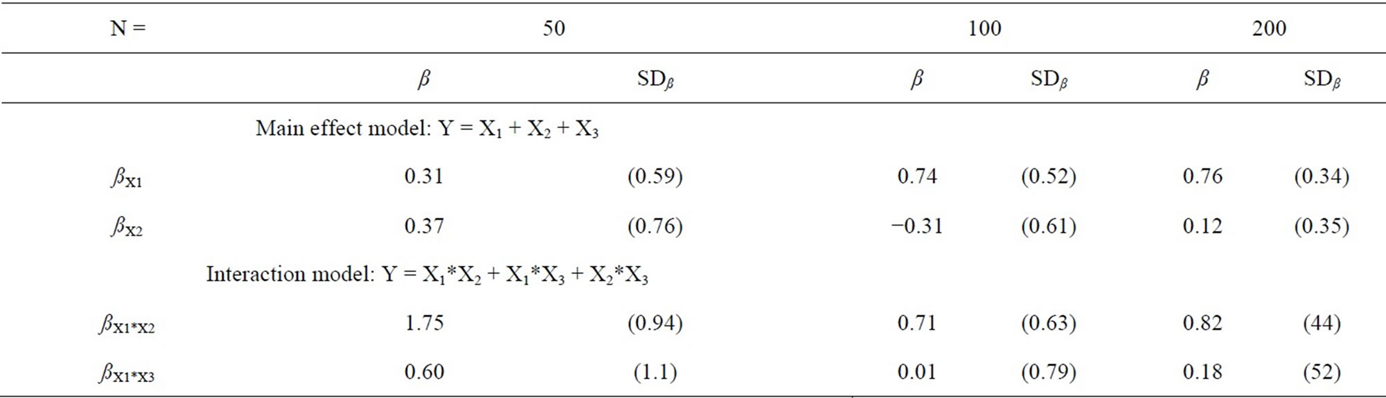
Table 2. Regression coefficients before substitution of missing data.
seven auxiliary variables because it is realistic to assume that an analyst would not merely include the variables of primary interest for the final analysis but would like to have some additional information available—for example should unexpected results turn up. The X-variables have a mean correlation of r = 0.39, with a range from 0.01 - 0.84. The simulations for main effects did not contain the interaction terms of the regression model, the simulations for the interaction models contained all underlying main effects. As can be seen in Table 2, the coefficients were reproduced comparatively well in the three different sample sizes, except for the main effects with n = 50, where the non-zero and the zero coefficient showed basically the same value. The random draw was kept nevertheless in order to avoid introducing spurious results. For each percentage of missing data, the estimation was repeated 200 times with a different starting value to estimate the variance due to the introduction of missing data. All simulations were performed up to 63% of missing data, or until the program broke down. The latter was partly the case because the imputations could not be performed, and partly because the logistic regression stopped. No attempt to force the programs was made after a breakdown. No missing data were replaced in the response variable, and all simulations were based on m = 5 multiple imputations of the dataset.
4. Results
Figure 1 shows the estimated β-coefficients over the 200
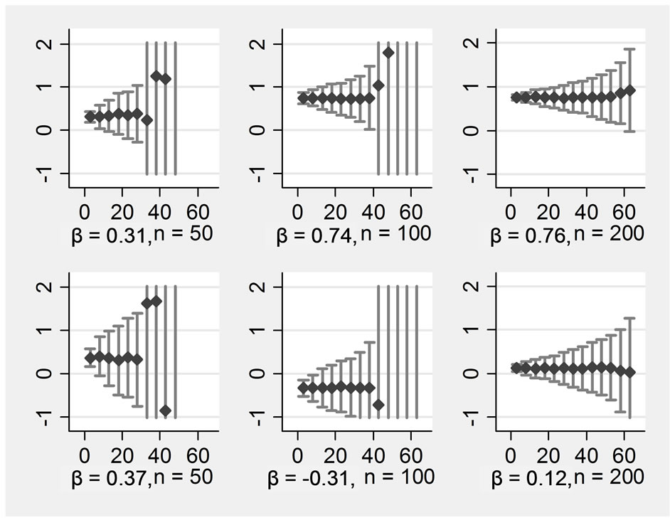
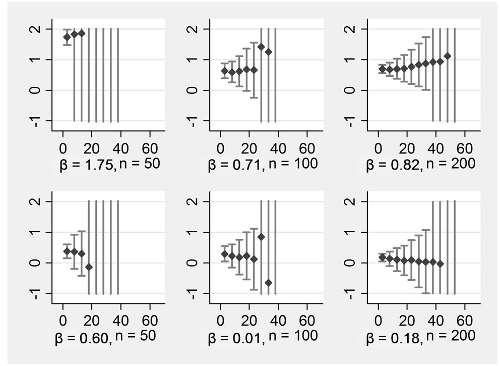
Figure 1. ß-regression coefficients (y-axis) for various proportions of missings (x-axis) in an imputation model with four variables Rows display: (1 left) ßx1, (2 left) ßx2, (1 right) ßx1*x2, (2 right) ßx1*x3, Columns display: (1) n = 50, (2) n = 100, (3) n = 200.
replications for each proportion of missing data for the main effects when only four variables were included into the imputation model (run 1 and 2). The upper row displays the non-zero main effects, the lower one the zero main effects. The columns display the sample sizes n = 50, n = 100, and n = 200. For better comparability, all Y-scales were restricted to the range from −1 to +2, Xscales represent the range of missing data in all Xs from 0% to 65%.
It can be seen that the simulation revealed generally unbiased estimates. However, the more missing data were introduced, the lower the precision of the estimates became. The distribution of the estimated coefficients was approximately normal. When 63% of data were missing, one would probably prefer not to perform any analysis with data from the present condition, the standard deviation lies around one then. This means that about one third of the observed regression coefficients would be much lower or higher than the true value. Regarding a main effect with a sample size of n = 200, we would recommend substituting no more than 40% of the missing data under the conditions simulated here. Regarding an interaction effect, the cut-off should be earlier. The two simulations with smaller sample sizes look even worse. With n = 100, the simulation results became completely imprecise when 42% of the data were missing, and we would suggest the following limit: imputations should be performed with a maximum of missing data of about 30%. With n = 50, the breakdown occurred at 33%, and whether to substitute if more than 20% of the data are missing in such a small sample should be considered carefully.
The pattern was positively influenced by including auxiliary variables into the substitution model. Figure 2 shows the results of the same data as before, but now the seven auxiliary variables have been included into the substitution model in addition to the four central variables. There was still no bias, and precision increased. In the smaller samples of n = 50 and n = 100, the breakdowns occurred at higher rates of missing data than without auxiliary variables. An analysis of the break-downs shows that single extreme outliers occurred here. For example, an extreme outlier for βX1 in n = 100 was observed when 63% of the data were missing, with a value of β = 927 (standard error = 400 000), the next extreme was 460 (standard error = 100 000). The occurrence of such extreme values was always associated with extreme standard errors. Even an estimate of β = 4 still had a standard error of 6000.
A different result was obtained for the interaction effects (see Figures 3). Including auxiliary variables did not improve the estimates very much. The problem here was not bias but rather precision. In the small sample of n = 50, a breakdown already occurred when 8% or 13% of the data were missing, and in larger samples, precision was considerably smaller than for main effects. Again, coefficients take on extreme values in the imputation for small samples with few variables when large proportions of data are missing.
Figure 3 shows a comparison of various programs utilizing the 4 variables. This was done solely for n = 100, because it was not expected that any program would be better for small or large samples specifically. Hence, results should be compared to the middle column of Figure 1. The first column displays the four regression coefficients when the imputation is performed using STATA’s ice but with the option “passive” selected. This means that the interaction terms were not used as predictors to impute the missing values of X1, X2 and X3. Such a specification makes sense intuitively. In the present example, results are considerably better than those obtained with the JAV method as used before. Hence, whenever possible,
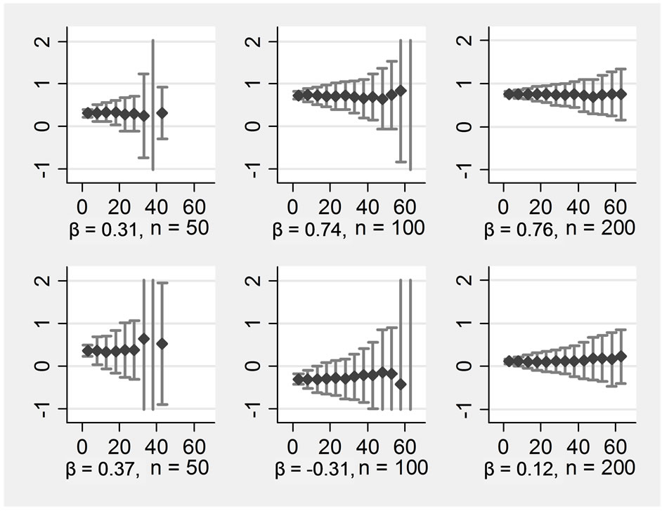
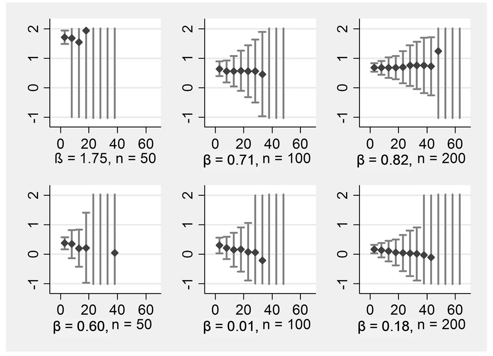
Figure 2. ß-regression coefficients (y-axis) for various proportions of missings (x-axis) in an imputation model with 11 variables Rows display: (1 left) ßx1, (2 left) ßx2, (1 right) ßx1*x2, (2 right) ßx1*x3, Columns display: (1) n = 50, (2) n = 100, (3) n = 200.
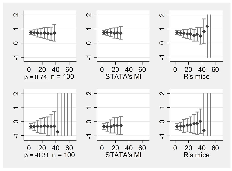
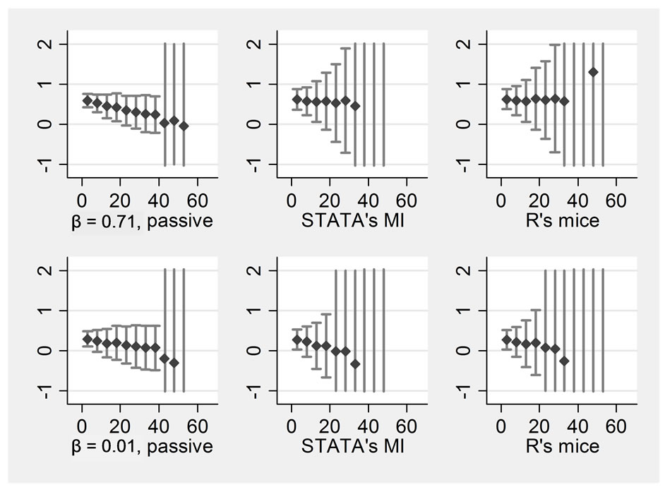
Figure 3. Passive imputation, STATA’s MI, R’s “mice” all n = 100, variables = 4 Rows display: ((1 left) ßx1, (2 left) ßx2, (1 right) ßx1*x2, (2 right) ßx1*x3, Columns display: (1) passive imputation using STATA’s ice, (2) STATA’s MI, (3) R’s mice.
the passive option should be selected. However, the JAV method has the advantage that it can be used with any program. The second column displays the results when STATA’s MI program was used. We specified “mi impute chained (pmm) variables” to receive results most comparable to “ice”. As the graph shows, differences between the two programs are negligible. The last column displays the results when R’s “mice” was selected to perform the imputations. The code used can be obtained from the first author. Here, we can see some advantages because mice would still produce results even with large amounts of missing data where STATA would fail. However, precision of the estimates is not higher.
The practical evaluation of the programs revealed that they were generally easy to handle, applications could be done in a few lines, and the time to learn the main features was a few hours. The time required to run the multiple imputations nonlinearly depended on the number of variables in the imputation model. With four variables, it took less than a second to create a single imputed dataset, with 30 it took several seconds and with 300 several hours (on a standard PC built in 2010). The number of imputed datasets linearly determined the running time. Sample size or proportion of missing data did not play a significant role. There were no relevant differences between “mice”, “STATA’s MI” and “ice”.
5. Discussion
With multiple imputations by chained equations, the statistician has a tool that can effectively eliminate missing data in a dataset and that can be very helpful in the analysis of data. In the present simulations, it resulted in unbiased estimates even when relatively large proportions of the data were missing, this held true for non-zero and zero coefficients, and for main effects as well as for interactions. However, depending on the proportion of missing data, a large amount of random variance became visible. Only a small amount of this variance stemmed from the imputation, the major part came from the missing data themself (data not shown).
The latter cannot be controlled by the researcher, and can lead to severe misinterpretation of the data. This is particularly the case for interaction effects, and the probability of estimating them precisely decreases drastically when large amounts of data are missing—and the one for finding false positive effects increases. The regular user will not perform 200 replications of an analysis, but only one. In addition, there is no possibility of comparing the results obtained with a dataset after imputation with those of a dataset without any missing data. As a result, we would recommend that the analyst should provide a table of descriptive statistics before the multiple imputation was performed when he publishes his data to enable the reader to estimate possible effects introduced by the imputation. There is no clear rule as to how much missing data can be substituted—under the present condition in a sample of n = 50 and only four variables, we would not recommend substituting more than about 20%, but in large samples with many variables and particularly when main effects are predominantly of interest, the proportions of missing data could be much higher.
Inclusion auxiliary variables can be beneficial, and in most data analyses it would be likely to occur. However, including too many auxiliary variables leads to over-parameterization, which will lead to a situation where all associations become biased downwards. In a previous study [23] we examined the effects of auxiliary variables in a linear regression analysis and recommended as a rule of thumb that the number of variables in the imputation model should not be larger than one third the number of cases that have observed data. Here, the effect of auxiliary variables was not explored systematically, but we would assume that this rule of thumb would also apply.
The choice of the program is not essential as long as there are missing data only in continuous variables. Missing data in binary variables or categorical variables with more than two categories will cause most programs to break down when samples are small or have many variables, in such cases mice would probably be the best choice. A situation where a researcher obtains a false result due to large outliers does not constitute a risk; the extreme standard error would be a clear warning for the researcher—given that he does not overlook it.
6. Conclusions
The present study has the following limitations. (1) As with any simulation, it is restricted to a certain range of situations. Reality is usually more complex. (2) We used a MCAR mechanism to introduce the missing data. Here, we did not find any bias. This is an important result, but cannot be generalized for MAR or even MNAR conditions. (3) We used a parameter of a logistic regression on an unevenly distributed response (14% yes, 86% no) as a single outcome. Other outcomes or other statistics may lead to different conclusions. However, there is a growing literature on how to deal with missing data in special problems, e.g. for Cox regression [37] or ROC-curve estimation [38]. (4) In these simulations, we intentionally pushed the imputation programs up to the point where they broke down. Clearly, a statistician should not go so far in a real data analysis. As we have demonstrated, the estimates with large amounts of missing data became so imprecise that a statistician should admit that there are situations where there is no way to analyse a certain dataset.
Given these caveats, multiple imputations by chained equations can be recommended for the analysis of data with missing values. As long as the proportion of missing data is moderate—say up to 20%—and only main effects are of interest, it can even be applied to small datasets like n = 50. Smaller datasets than n = 50 are not suitable for regression analysis anyway, so no conclusion about them can be drawn from the present study. When interactions are to be analysed, larger datasets are needed. Making use of the “passive” option can improve the estimate drastically. Since the implementation of multiple imputation is relatively easy, and the time to run the imputation on a modern computer seldom exceeds one night, they can be recommended for the imputation of moderate amounts of missing data without any restrictions. When there are larger amounts of missing data, multiple imputation is still a method of choice, but only for larger sample sizes. Additionally, some drawbacks have to be taken into account. In small samples, it is questionable whether the benefits of such an analysis outweigh the risks. For very simple analyses, e.g. main effect models, it may still be applied. For more sophisticated analyses, it will carry a high risk of drawing false conclusions.
7. Acknowledgements
This work was supported by the Stiftung Rheinland-Pfalz für Innovation (959).
REFERENCES
- J. Hardt and K. Görgen, “Multiple Imputation Using ICE: A Simulation Study on a Binary Response,” 6th German Stata User Group Meeting, Berlin, 2008. http://www.stata.com/meeting/germany08/abstracts.html
- J. W. Graham, S. M. Hofer and A. M. Piccinin, “Analysis with Missing Data in Drug Prevention Research,” NIDA Research Monography, Vol. 142, 1994, pp. 13-63.
- S. van Buuren, “Multiple Imputation of Discrete and Continuous Data by Fully Conditional Specification,” Statistical Methods in Medical Research, Vol. 16 No. 3, 2007, pp. 219-242. http://dx.doi.org/10.1177/0962280206074463
- G. Papastenafou and M. Wiedenbeck, “Singuläre und Multiple Imputation Fehlender Einkommenswerte. Ein Empirischer Vergleich,” ZUMA Nachrichten, Vol. 43, 1998, pp. 73-89.
- G. J. van der Heijden, A. R. Donders, T. Stijnen and K. G. Moons, “Imputation of Missing Values Is Superior to Complete Case Analysis and the Missing-Indicator Method in Multivariable Diagnostic Research: A Clinical Example,” Journal of Clinical Epidemiology, Vol. 59, No. 10, 2006, pp. 1102-1109. http://dx.doi.org/10.1016/j.jclinepi.2006.01.015
- D. B. Rubin, “Multiple Imputation for Nonresponse in Surveys,” Wiley & Sons, New York, 1987. http://dx.doi.org/10.1002/9780470316696
- X. L. Meng, “Multiple-Imputation Inferences with uncongenial Sources of Input,” Statistical Science, Vol. 9, No. 4, 1994, pp. 538-573.
- P. S. Albert, “Imputation Approaches for Estimating Diagnostic Accuracy for Multiple Tests from Partially Verified Designs,” Biometrics, Vol. 63, No. 3, 2007, pp. 947- 957. http://dx.doi.org/10.1111/j.1541-0420.2006.00734.x
- S. A. Barnes, S. R. Lindborg and J. W. Seaman Jr., “Multiple Imputation Techniques in Small Sample Clinical Trials,” Statistics in Medicine, Vol. 25, No. 2, 2006, pp. 233-245. http://dx.doi.org/10.1002/sim.2231
- O. Harel and X. H. Zhou, “Multiple Imputation: Review of Theory, Implementation and Software,” Statistics in Medicine, Vol. 26, No. 16, 2007, pp. 3057-3077. http://dx.doi.org/10.1002/sim.2787
- D. B. Rubin, “Multiple Imputations after 18 plus Years,” Journal of the American Statistical Association, Vol. 91, No. 434, 1996, pp. 473-489. http://dx.doi.org/10.1080/01621459.1996.10476908
- A. R. Donders, G. J. van der Heijden, T. Stijnen and K. G. Moons, “Review: A Gentle Introduction to Imputation of Missing Values,” Journal of Clinical Epidemiology, Vol. 59, No. 10, 2006, pp. 1087-1091. http://dx.doi.org/10.1016/j.jclinepi.2006.01.014
- J. L. Schafer and J. W. Graham, “Missing Data: Our View of the State of the Art,” Psychological Methods, Vol. 7, No. 2, 2002, pp. 147-177. http://dx.doi.org/10.1037/1082-989X.7.2.147
- C. Bono, L. D. Ried, C. Kimberlin and B. Vogel, “Missing Data on the Center for Epidemiologic Studies Depression Scale: A Comparison of 4 Imputation Techniques,” Research in Social and Administrative Pharmacy, Vol. 3, No. 1, 2007, pp. 1-27. http://dx.doi.org/10.1016/j.sapharm.2006.04.001
- F. M. Shrive, H. Stuart, H. Quan and W. A. Ghali, “Dealing with Missing Data in a Multi-Question Depression Scale: A Comparison of Imputation Methods,” BMC Medical Research Methodology, Vol. 6, No. 57, 2006. http://www.ncbi.nlm.nih.gov/entrez/query.fcgi?cmd=Retrieve&db=PubMed&dopt=Citation&list_uids=17166270 http://dx.doi.org/10.1186/1471-2288-6-57
- N. J. Horton and K. P. Kleinman, “Much Ado about Nothing: A Comparison of Missing Data Methods and Software to Fit Incomplete Data Regression Models,” American Statistician, Vol. 61, No. 1, 2007, pp. 79-90. http://dx.doi.org/10.1198/000313007X172556
- R. J. Little, M. Yosef, K. C. Cain, B. Nan and S. D. Harlow, “A Hot-Deck Multiple Imputation Procedure for Gaps in Longitudinal Data on Recurrent Events,” Statistics in Medicine, Vol. 27, No. 1, 2008, pp. 103-120. http://dx.doi.org/10.1002/sim.2939
- J. Siddique and T. R. Belin, “Multiple Imputation Using an Iterative Hot-Deck with Distance-Based Donor Selection,” Statistics in Medicine, Vol. 27, No. 1, 2008, pp. 83- 102. http://dx.doi.org/10.1002/sim.3001
- P. Royston, “Multiple Imputation of Missing Data: Update,” Stata Journal, Vol. 5, No. 4, 2005, pp. 188-201.
- P. Royston, “Multiple Imputation of Missing Data,” Stata Journal, Vol. 4, No. 3, 2004, pp. 227-241.
- J. W. Graham, A. E. Olchowski and T. D. Gilreath, “How Many Imputations Are Really Needed? Some Practical Clarifications of Multiple Imputation Theory,” Prevention Science, Vol. 8, No. 3, 2007, pp. 206-213. http://dx.doi.org/10.1007/s11121-007-0070-9
- A. Marshall, D. G. Altman, R. L. Holder and P. Royston, “Combining Estimates of Interest in Prognostic Modelling Studies after Multiple Imputation: Current Practice and Guidelines,” BMC Medical Research Methodology, Vol. 9, No. 57, 2009. http://www.ncbi.nlm.nih.gov/entrez/query.fcgi?cmd=Retrieve&db=PubMed&dopt=Citation&list_uids=21194416 http://dx.doi.org/10.1186/1471-2288-9-57
- J. Hardt, M. Herke and R. Leonhart, “Auxiliary Variables in Multiple Imputation in Regression with Missing X: A Warning against Including Too Many in Small Sample Research,” BMC Medical Research Methodology, Vol. 12, No. 184, 2012. http://www.biomedcentral.com/1471-2288/12/184 http://dx.doi.org/10.1186/1471-2288-12-184
- G. Ambler, R. Z. Omar and P. Royston, “A Comparison of Imputation Techniques for Handling Missing Predictor Values in a Risk Model with a Binary Outcome,” Statistical Methods in Medical Research, Vol. 16, No. 3, 2007, pp. 277-298. http://dx.doi.org/10.1177/0962280206074466
- P. Royston, “Multiple Imputation of Missing Data: Update of Ice,” Stata Journal, Vol. 5, No. 4, 2005, pp. 527- 536.
- K. Groothuis-Oudshoorn and S. van Buuren, “Mice: Multivariate Imputation by Chained Equations in R,” Journal of Statistical Software, Vol. 45, No. 3, 2011. http://www.jstatsoft.org/v45/i03
- S. van Buuren, H. C. Boshuizen and D. L. Knook, “Multiple Imputation of Missing Blood Pressure Covariates in Survival Analysis,” Statistics in Medicine, Vol. 18, No. 6, 1999, pp. 681-694. http://dx.doi.org/10.1002/(SICI)1097-0258(19990330)18:6<681::AID-SIM71>3.0.CO;2-R
- A. Gelman, G. King and C. Liu, “Not Asked and Not Answered: Multiple Imputation for Multiple Surveys,” Journal of the American Statistical Association, Vol. 93, No. 443, 1998, pp. 846-855. http://dx.doi.org/10.1080/01621459.1998.10473737
- S. R. Seaman, J. W. Bartlett and I. R. White, “Multiple Imputation of Missing Covariates with Non-Linear Effects and Interactions: An Evaluation of Statistical Methods,” BMC Medical Research Methodology, Vol. 12, No. 46, 2012. http://www.ncbi.nlm.nih.gov/entrez/query.fcgi?cmd=Retrieve&db=PubMed&dopt=Citation&list_uids=22489953 http://dx.doi.org/10.1186/1471-2288-12-46
- S. van Buuren, “Flexible Imputation of Missing Data,” CRC Press (Chapman & Hall), Boca Raton, 2012. http://dx.doi.org/10.1201/b11826
- P. Royston, “Multiple Imputation of Missing Data: Update,” Stata Journal, Vol. 5, No. 2, pp. 188-201.
- J. Hardt, U. T. Egle and J. G. Johnson, “Suicide Attempts and Retrospective Reports about Parent-Child Relationships: Evidence for the Affectionless Control Hypothesis,” GMS—Psycho-Social-Medicine, 2007. http://www.egms.de/en/journals/psm/2007-4/psm000044.shtml
- U. T. Egle and J. Hardt, “MSBI: Mainz Structured Biographical Interview (MSBI: Mainzer Strukturiertes Biografisches Interview),” In: B. Strauss and J. Schumacher, Eds., Klinische Interviews und Ratingskalen. Diagnostik für Klinik und Praxis (Band 4), 2004, Göttingen, Hogrefe, pp. 261-265.
- J. Hardt, U. T. Egle and A. Engfer, “Der Kindheitsfragebogen, ein Instrument zur Beschreibung der Erlebten Kindheitsbeziehungen zu den Eltern,” Zeitschrift fuer Differentielle und Diagnostische Psychololgie, Vol. 24, No. 1, 2003, pp. 33-43. http://dx.doi.org/10.1024//0170-1789.24.1.33
- J. Hunzinger, U. T. Egle, G. Vossel and J. Hardt, “Stabilität und Stimmungsabhängigkeit Retrospektiver Berichte zu Eltern-Kind-Beziehungen,” Zeitschrift fuer Klinische Psychologie und Psychotherapie, Vol. 36, No. 4, 2007, pp. 235-242. http://dx.doi.org/10.1026/1616-3443.36.4.235
- C. E. Enders, “Applied Missing Data Analysis,” Guilford, New York, 2010.
- A. Marshall, D. G. Altman and R. L. Holder, “Comparison of Imputation Methods for Handling Missing Covariate Data When Fitting a Cox Proportional Hazards Model: A Resampling Study,” BMC Medical Research Methodology, Vol. 10, No. 112, 2010. http://www.ncbi.nlm.nih.gov/entrez/query.fcgi?cmd=Retrieve&db=PubMed&dopt=Citation&list_uids=21194416 http://dx.doi.org/10.1186/1471-2288-10-112
- Y. An, “Smoothed Empirical Likelihood Inference for ROC Curves with Missing Dat,” Open Journal of Statistics, Vol. 2012, No. 2, 2012, pp. 21-27. http://www.SciRP.org/journal/ojs http://dx.doi.org/10.4236/ojs.2012.21003
NOTES
*An early draft of this paper was published by Hardt, J. and Görgen, K. [1].
1The original analysis included a simulation with n = 400. However, results did not differ very much from those obtained with n = 200 so that we decided to omit presenting them here. Interested readers can obtain them from JH.