American Journal of Computational Mathematics
Vol.06 No.03(2016), Article ID:71024,11 pages
10.4236/ajcm.2016.63029
Adaptive Finite Element Method for Steady Convection-Diffusion Equation
Gelaw Temesgen Mekuria1, Jakkula Anand Rao2
1Department of Mathematics, Mizan Tepi University, Mizan Teferi, Ethiopia
2Department of Mathematics, Osmania University, Hyderabad, India

Copyright © 2016 by authors and Scientific Research Publishing Inc.
This work is licensed under the Creative Commons Attribution International License (CC BY).
http://creativecommons.org/licenses/by/4.0/


Received 24 June 2016; accepted 27 September 2016; published 30 September 2016
ABSTRACT
This paper examines the numerical solution of the convection-diffusion equation in 2-D. The solution of this equation possesses singularities in the form of boundary or interior layers due to non-smooth boundary conditions. To overcome such singularities arising from these critical regions, the adaptive finite element method is employed. This scheme is based on the streamline diffusion method combined with Neumann-type posteriori estimator. The effectiveness of this approach is illustrated by different examples with several numerical experiments.
Keywords:
Convection-Diffusion Problem, Streamline Diffusion Finite Element Method, Boundary and Interior Layers, A Posteriori Error Estimators, Adaptive Mesh Refinement

1. Introduction
This paper deals with the scalar convection-diffusion equation. This equation describes the transport of scalar quantity, e.g., temperature or concentration. We are interested in the convection dominated case. In this case, the solution of a convection-diffusion equation frequently has boundary or interior layers. It is well known that the standard Galerkin finite element discretization on uniform grids produces inaccurate oscillatory solutions to convection diffusion problems. Therefore several stabilized finite element methods have been developed, e.g., the streamline-upwind Petrov-Galerkin (SUPG) method [1] & [2] or streamline-diffusion finite element method (SDFEM) [3] is designed to overcome these problems by introducing a small amount of artificial diffusion in the direction of streamlines. The numerical solution obtained from the SDFEM has the desirable property that the accuracy in regions where the exact solution is smooth will not be degraded as a result of discontinuities and layers in the exact solution [4] & [5] . However, the numerical solution obtained from the SDFEM can be oscillatory in regions where there are layers. One common technique to increase the accuracy of the finite element solution in these critical regions is through local grid refinement, the so-called h-method. The question is how to identify those regions and how to obtain a good balance between the refined and unrefined regions such that the overall accuracy is optimal.
Another related problem is to obtain reliable estimates of the accuracy of the computed numerical solution. A priori estimate are often insufficient and can’t be used to estimate the exact error. Therefore, it is natural to acquire a posteriori error estimators to pinpoint where the error is large and, at the same time, properly bound the exact error on the whole domain. The error estimator should be local and should yield reliable upper and lower bounds for the true error in a user-specified norm. Global upper bounds are sufficient to obtain a numerical solution with accuracy below a prescribed tolerance. Local lower bounds are necessary to ensure that the grid is correctly refined so that one obtains a numerical solution with a prescribed tolerance using a nearly minimal number of grid-points.
For two-dimensional problems, several estimators have been shown to be asymptotically exact when used on uniform meshes provided the solution of the problem is smooth enough [6] - [8] . Estimators based on computing residuals, so-called residual-type estimators, and estimators based on solving a local Dirichlet problem, so-called Dirichlet-type estimators, were introduced in [9] . Estimators based on solving a local Neumann problem, so- called Neumann-type estimators, were first given in [10] . These estimators have been studied by many researchers in [11] - [16] . The Zienkiewicz-Zhu (ZZ) type of estimators based on recovery of gradient and Hessian are also well developed, see [17] & [18] , and articles cited therein.
In this paper we introduce and analyze from theoretical and experimental points of view an adaptive scheme to efficiently solve the convection-diffusion equation. This scheme is based on the streamline-diffusion finite element method (SDFEM) introduced in [3] combined with an error estimator similar to the one developed in [14] . We prove global upper and local lower error estimates in the energy norm, with constants which only depend on the shape-regularity of the mesh and the polynomial degree of the finite element approximating space. We perform several numerical experiments to show the effectiveness of our approach to capture boundary and inner layers sharply and without significant oscillations.
The paper is organized as follows. In Section 2 we recall the convection-diffusion problem under consideration and the Streamline Diffusion Finite Element Method. In Section 3 we define a posteriori error estimator with the energy norm of the finite element approximation error. Finally, in Section 4, we introduce the adaptive scheme and report the results of the numerical tests.
2. Linear Convection-Diffusion Equation
We consider the following steady linear convection-diffusion equation
 , (2.1a)
 , and (2.1b)
 (2.1c)
where  is a bounded polygonal domain with Lipschitz boundary
  and
and . We are interested in the convection dominated case and assume that
(A.1) ,
,
(A.2) ,
,
(A.3) ,
,
(A.4) .
.
The  norm and the
  semi-norm (also called Energy Norm) are defined as
 and (2.2)
 (2.3)
(2.3)
 , respectively. We shall denote the above norm and semi-norm by the following convention
 and
and  if no subscript index is given then we assume an ordinary
norm,  , and if no subscript index is given then we shall assume it is the whole of
 .
.
To define weak form of Equation (2.1), we need two classes of functions: the trial functions  and the test solutions
 :
:
 (2.4)
(2.4)
 (2.5)
(2.5)
The standard variational formulation of Equation (2.1) is given by: Find  such that
 (2.6)
(2.6)
where
 and (2.7)
 (2.8)
(2.8)
Let  be a decomposition of
  into triangles.
We need to make the following geometrical assumptions on the family of triangulations 
1) Admissibility: whenever  and
and  belongs to
 ,
,  is either empty, or reduced to a common vertex, or to a common edge
1)  = the diameter of K = the longest side of
3)  = the supremum of the diameter of the balls inscribed in
4) Shape regularity: the ratio of  to
to  is uniformly bounded i.e.,
 (2.9)
(2.9)
which means for any  and for any
  there exists a constant
  such that
  where
where  denotes the smallest angle in any
 .
.
We define the finite element spaces
 (2.10)
for triangular elements, where  is the space of polynomials of degree not greater than 1 on K.
In the case of convection-dominated problem, the standard Galerkin approximation of Equation (2.6) may produce unphysical behavior, oscillation, if the mesh is too coarse in critical regions. To circumvent these difficulties, stability of the discretization has to be increased by introducing artificial diffusion along streamlines. The Streamline-Diffusion Finite Element Method (SDFEM) [1] - [3] stabilizes a convection-dominated problem by adding weighted residuals to the standard Galerkin finite element method for hyperbolic equations which combines good stability with high order accuracy, convergence results are available (see [19] ).
The SDFEM yields the following discrete problem obtained: Find  such that
 (2.11)
where
 and (2.12)
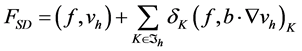 (2.13)
In Equation (2.11), a constant  must be chosen for every element K. Let the mesh Peclet number be de-
fined by,  where
where  denotes the norm in
 . From the analysis of the SDFEM, the
following choice of  are optimal; see [20] :
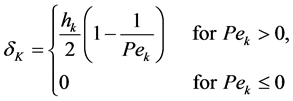 (2.14)
where  is a measure of the element length in the direction of the convection flow b. For other parameter choice, see [21] - [24] .
3. A Posteriori Error Estimator
In this topic, we introduce the analysis of a Neumann-type error estimator proposed in [14] which is an extension of the work [25] . In their work, they modify the well-known Bank and Weiser estimator [10] and using the idea of Ainsworth & Oden in [26] , they solve a local (element) Poisson problem over a suitably chosen (higher order) approximation space with data from interior residuals and flux jumps along element edges.
We now introduce some definitions and notations that will be needed for the error estimates.
We denote by  the set of edges of element
 , by
, by  the set of all element edges
and the subsets relating to internal, Dirichlet and Neumann edges respectively as
 ,
,  and
and
 so that
 .
.
We denote  the set of vertices of
  and by
  the set of all element vertices (that
do not lie on the Dirichlet boundary ). Let
  be the set of vertices of
 , and for
 ,
,  and
and  we define the local “patches” of elements as
 ,
,  ,
,  ,
, 
For the lowest order  approximations over a triangular element subdivision,
  , so that the interior residual of element K is given by
 (3.1)
(3.1)
and the internal residual is approximated by
 (3.2)
(3.2)
where  is the
  -projection onto
 .
.
For any edge  of an element
 , we define the flux jump as
 (3.3)
(3.3)
where  is a constant function on the inter-element edge
  and
and  measures the jump of
across , that is, for
 ,
,  and defining
  and
and  to be the outward normals with respect to the edge
  from element K and S respectively, we have
 (3.4)
(3.4)
The approximation space is denoted by
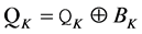 (3.5)
(3.5)
consisting of edge and interior bubble functions respectively:
 (3.6)
(3.6)
where each member of the space is a quadratic (or biquadratic) edge bubble function  that is nonzero on edge E of element K, but non zero valued on all other edges of K.
 is the space spanned by interior cubic (or biquadratic) bubbles
  i.e.,
i.e.,
 (3.7)
(3.7)
where each function is associated with an element K, and is zero on all edges of K, nonzero on the interior of K, and  at the centeroid of K.
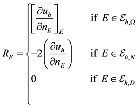
The upshot is that the local problems are always well posed and that for each triangular element a 4 × 4 system of equations must be solved to compute .
.
For an element , the local error estimate is the energy norm of
  given by
 (3.8)
(3.8)
where  satisfies
 (3.9)
(3.9)
In the following, we use the short-hand notation  to denote
  -norm of a function
 . The Kay and Silvester’s a posteriori error estimation can be read as following:
Theorem 1. If the variational Equation (2.6) solved with a grid of linear triangular elements, and if the triangle aspect ratio condition is satisfied with , then, the estimator
  computed via Equation (3.9) satisfies the (global) upper bound property
 (3.10)
where C is independent of  and h and
  is the length of the longest edge of element K.
Proof. See the details in [14] .
Theorem 2. If the variational Equation (2.6) with  is solved via either the Galerkin formulation or the SD formulation Equation (2.11), using a grid of linear triangular elements, and if the triangle aspect ratio condition is satisfied, then the estimator
  computed via Equation (3.9) is a local lower bound for
  in the sense that
 (3.11)
where c is independent of , and
, and  represents the patch of four elements that have at least one boundary edge E from the set
 .
.
Proof. See the details in [14] .
4. Numerical Experiments
In this section we report three series of numerical experiments with the Streamline Diffusion stabilization method described in Section (2) and an h-adaptive mesh-refinement strategy based on the error estimator analyzed in Section (3). In all the experiments we have used piecewise linear finite elements (i.e.,  polynomial degree
 ) and we have taken as geometric domain the unit square
  or
or , although with different boundary conditions. We have considered varying values of the coefficients
 ,
,  , and
, and  of the convection-diffusion equation.
The adaptive procedure consists in solving Equation (2.11) on a sequence of meshes up to finally attain a solution with an estimated error within a prescribed tolerance. To attain this purpose, we initiate the process with a quasi-uniform mesh and, at each step, a new mesh better adapted to the solution of Equation (2.6) must be created. This is done by computing the local error estimators  for all K in the “old” mesh
 , and refining
those elements K* with , where
  is a prescribed parameter. In all our expe-
riments we have chosen . For other marking strategies, we refer to [27] .
The implementation used in this paper is derived from iFEM [28] . This software package is the successor of AFEM@MATLAB [29] , which contains an advanced refinement tool.
Example 1 (Exponential boundary layer) The first test problem contains an exponential boundary layer. This
problem corresponds to the case of , zero forcing
 , Dirichlet boundary condition,
  and
and
the exact solution is given by
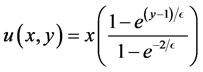 (4.1)
(4.1)
We report the results obtained for  and
and  over the domain
 .
.
Figure 1 shows the successfully refined meshes created in the adaptive process for , as well as the corresponding computed solution. Figure 2 shows the error curves for the exact and estimated errors. Figure 3
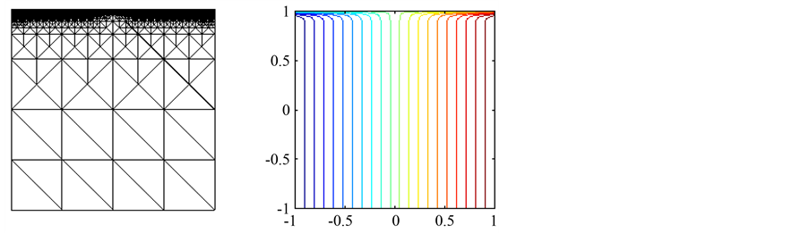
Figure 1. Adaptive grids (left) and solution (right) obtained for  & d.o.f:3663.
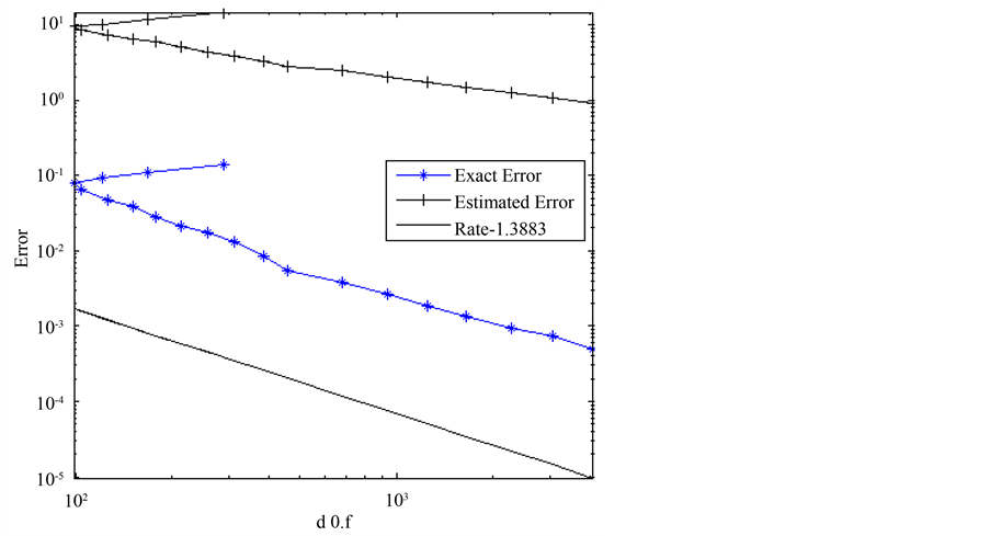
Figure 2. Estimated and exact error curves using .
.
and Figure 4 show analogous results for the same problem with the parameter . The results show that the estimated error is well bounded as described in [22] .
Example 2 (Interior layers) We consider Equation (2.1) with  and
and ,
,  ,
, . The forcing term f and boundary condition are determined from the exact solution:
 (4.2)
(4.2)
Figure 5 and Figure 6 clearly show that the adaptive method has successfully refined the correct elements using a greater concentration of elements in the interior layer. Figure 7 and Figure 8 show the estimated and exact error curves decrease monotonically for  and
and  respectively.
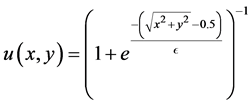
Example 3 (Interior and boundary layers) We consider Equation (2.1) with ,
,
 ,
,  and boundary conditions
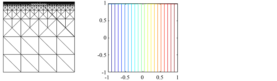
Figure 3. Adaptive grids (left) and solution (right) obtained for  & d.o.f: 4183.
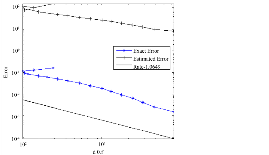
Figure 4. Estimated and exact error curves using .
.
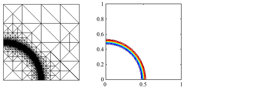
Figure 5. Adaptive grids (left) and solution (right) obtained for  & d.o.f:5523.
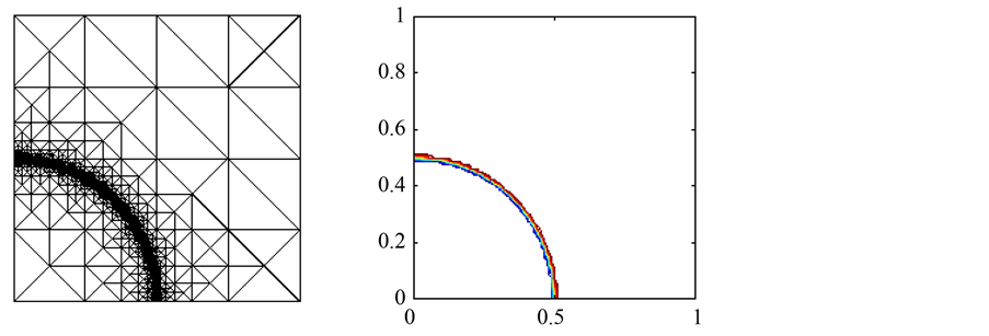
Figure 6. Adaptive grids (left) and solution (right) obtained for  with d.o.f:6259.
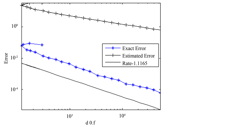
Figure 7. Estimated and exact error curves using .
.
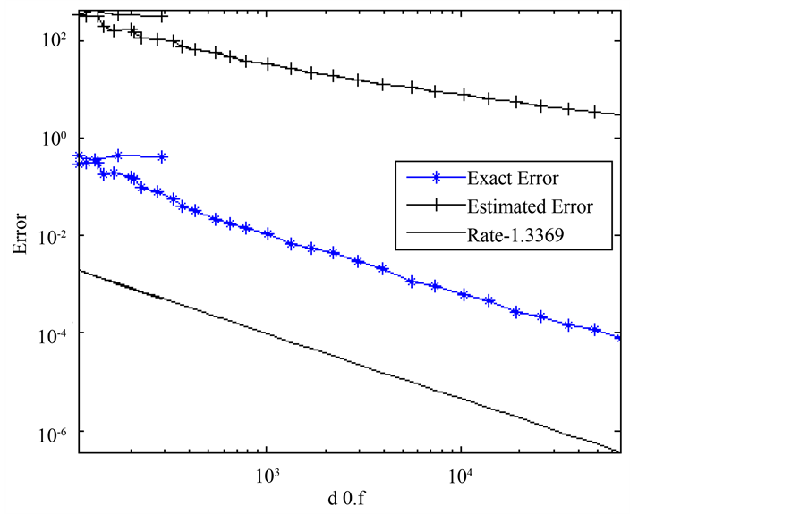
Figure 8. Estimated and exact error curves using .
.
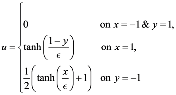 (4.3)
(4.3)
Discontinuities at  causes u to have an internal layer of width
  along the line
 , with values
  to the left and
  to the right, as well as a boundary layer along the outflow boundary. We do not include error curves because no analytical solution is known in this case.
Figure 9 and Figure 10 show some of the successively refined meshes created in the adaptive process for  and
and , as well as the corresponding computed solution.
In the case of  in Example (2) and
  in Example (3), the adaptive refinement process able to resolve the boundary and interior layers.
For the case of  in Example (2) and
  in Example (3), it is hard to fully resolve the internal layers and the numerical solution display a small oscillatory pattern in the internal layer.
5. Conclusions
An adaptive finite element scheme for the convection-diffusion equation has been introduced and analyzed. This scheme is based on the Streamline Diffusion Finite element method combined with a Neumann-type error estimator.
Several numerical experiments are reported. For , all of them show the effectiveness of this scheme to capture boundary and inner layers very sharply and without significant oscillations. But in the case of
  in Example (2) and
  in Example (3), the numerical solution displays small oscillatory pattern in the internal layer which requires a high computing cost to produce an accurate internal layer. In general, it is

Figure 9. Adaptive grids (left) and solution (right) obtained for  with d.o.f:34,897.

Figure 10. Adaptive grids (left) and solution (right) obtained for  with d.o.f:41,149.
quite evident that our error estimator provides an effective refinement indicator even in the presence of internal layers.
Cite this paper
Galeage Kaelo,Brothers Wilright Malema,Gelaw Temesgen Mekuria,Jakkula Anand Rao, (2016) Adaptive Finite Element Method for Steady Convection-Diffusion Equation. American Journal of Computational Mathematics,06,275-285. doi: 10.4236/ajcm.2016.63029
References
- 1. Central Statistics Office (2008) Botswana AIDS Impact Survey III: Statistical Report. Central Statistics Office, Gaborone.
- 2. Lamptey, P. and Price, J. (1998) Social Marketing Sexually Transmitted Disease and HIV Prevention; A Consumer-Centered Approach to Achieving Behaviour Change. AIDS, 12, S1-S9.
- 3. Bond, V. and Dover, P. (1997) Men, Women and the Trouble with Condoms: Problems Associated with Condom Use by Migrant Workers in Rural Zambia. Health Transition Review, 7, 377-391.
- 4. UNAIDS (2005) Report on the Global AIDS Epidemic. UNAIDS, Geneva.
- 5. WHO (2005) Newsletter, June. WHO, Geneva.
- 6. WHO (2000) Reproductive Health Report. WHO, Geneva.
- 7. Gollub, P. and Erica, L. (2000) The Female Condom: Tool for Women’s Empowerment. American Journal of Public Health, 90, 1377-1381.
http://dx.doi.org/10.2105/AJPH.90.9.1377 - 8. UNAIDS (2000) Report on the Global AIDS Epidemic: A UNAIDS 10th Anniversary Special Edition. UNAIDS, Geneva.
- 9. UNAIDS (1999) Report on the Global AIDS Epidemic. UNAIDS, Geneva.
- 10. Mmegi Newspaper (2010) Female Condom Not So Blissful. Mmegi Newspaper, 27, 26 April 2010.
- 11. AIDSCAP (1997) The Female Condom: From Research to the Market Place. United States of America.
- 12. WHO (2000) Sentinel Surveillance for HIV Infection: A Method to Monitor HIV Infection Trends in Population Groups. WHO, Geneva.
- 13. Hogan, P. and Kitagwa, M. (1985) The Impact of Social Status on Family Structure. American Sociological Review, 59, 408-424.
- 14. Brewster, K. (1994) Race Differences in Sexual Activity among Women. American Sociological Review, 59, 408-424.
http://dx.doi.org/10.2307/2095941 - 15. Meekers, D. and Richter, K. (2005) Factors Associated With Use of the Female Condom in Zimbabwe. International Family Planning Perspectives, 31, 30-37.
http://dx.doi.org/10.1363/3103005 - 16. Gilbert, M., Middlestadt, S. and Eustace, A. (2000) Using a KAPB Survey to Identify Determinants of Condom Use Among Sexually Active Adults. Journal of Applied Psychology, 25, 1-20.
- 17. Harrison, D., David, S., Riehman, K. and Eberstein, I. (1997) Factors Associated With Use of the Female Condom. Family Planning Perspectives, 29, 181-184.
http://dx.doi.org/10.2307/2953383 - 18. Macaluso, M., Artz, L., Fleenor, M., Robey, L., Kelaghan, J. and Cabral, R. (1997) Female Condom Use among Women at High Risk of Sexually Transmitted Diseases. Family Planning Perspective, 32, 138-44.
http://dx.doi.org/10.2307/2648163 - 19. Choi, K., Hoff, C., Gregorich, E. and Gomez, C. (2008) The Efficacy of Female Condom Skills Training in HIV Risk Reduction among Women: A randomized Controlled Trial. American Journal of Public Health, 98, 1841-1848.
http://dx.doi.org/10.2105/AJPH.2007.113050 - 20. Kenneth, S. and Hsiao, C. (2005) Multinomial Logit Specification Tests. International Economic Review, 26, 619-627.
- 21. Schmidt, P. and Strauss, R. (1975) The Prediction of Occupation Using Multinomial Logit Models. International Economic Review, 16, 471-486
- 22. Martin, S. (2008) AIDS and Behavioral Change to Reduce Risk: A Review. American Journal of Public Health, 78, 394-410.
- 23. Fapohunda, O. (2009) Reproductive Health Risk and Protective Factors among Youth in Lusaka, Zambia. Journal of Adolescent Health, 30, 76-86.
- 24. Dominik, M. and Trussell, A. (2004) Determinants of Condom Use among Young People. Studies in Family Planning, 33, 335-346.
- 25. Hughes, T.J.R. and Brooks, A.N. (1979) A Multidimensional Upwind Scheme with no Crosswind Diffusion. In: Hughes, T.J.R, Ed., Finite Element Methods for Convection Dominated Flows, AMD, Vol. 34, ASME, New York, 19-35.
- 26. Hughes, T.J.R., Mallet, M. and Mizukami, A. (1986) A New Finite Element Formulation for Computational Fluid Dynamics: II. Beyond SUPG. Computer Methods in Applied Mechanics and Engineering, 54, 341-355.
- 27. Johnson, C., Nävert, U. and Pitkäranta, J. (1984) Finite Element Methods for Linear Hyperbolic Equations. Computer Methods in Applied Mechanics and Engineering, 45, 285-312.
- 28. Roos, H.-G., Stynes, M. and Tobiska, L. (1996) Numerical Methods for Singularly Perturbed Differential Equations. Springer-Verlag, Berlin.
http://dx.doi.org/10.1007/978-3-662-03206-0 - 29. Johnson, C., Schatz, A.H. and Wahlbin, L.B. (1987) Crosswind Smear and Pointwise Errors in Streamline Diffusion Finite Element Methods. Mathematics of Computation, 49, 25-38.
http://dx.doi.org/10.1090/S0025-5718-1987-0890252-8 - 30. Babuška, I., Durán, R. and Rodríguez, R. (1992) Analysis of the Efficiency of an a Posteriori Error Estimator for Linear Triangular Finite Element. SIAM Journal on Numerical Analysis, 29, 947-964.
http://dx.doi.org/10.1137/0729058 - 31. Durán, R., Muschietti, M.A. and Rodríguez, R. (1991) On the Asymptotic Exactness of Error Estimators for Linear Triangular Finite Elements. Numerische Mathematik, 59, 107-127.
http://dx.doi.org/10.1007/BF01385773 - 32. Durán, R. and Rodríguez, R. (1992) On the Asymptotic Exactness of Bank-Weiser’s Estimator. Numerische Mathematik, 62, 297-303.
http://dx.doi.org/10.1007/BF01396231 - 33. Babuška, I. and Rheinboldt, W.C. (1978) Error Estimates for Adaptive Finite Element Computations. SIAM Journal on Numerical Analysis, 15, 736-754.
http://dx.doi.org/10.1137/0715049 - 34. Bank, R.E. and Weiser, A. (1985) Some a Posteriori Error Estimators for Elliptic Partial Differential Equations. Mathematics of Computation, 44, 283-301.
http://dx.doi.org/10.1090/S0025-5718-1985-0777265-X - 35. Ainsworth, M. and Babuška, I. (1999) Reliable and Roubst a Posteriori Error Estimation for Singular Perturbed Reaction-Diffusion Problems. SIAM Journal on Numerical Analysis, 36, 331-353.
http://dx.doi.org/10.1137/S003614299732187X - 36. Eriksson, K. and Johnson, C. (1993) Adaptive Streamline Diffusion Finite Element Methods for Stationary Convection-Diffusion Problems. Mathematics of Computation, 60, 167-188.
http://dx.doi.org/10.1090/S0025-5718-1993-1149289-9 - 37. Johnson, C. (1989) The Streamline Diffusion Finite Element Method for Compressible and Incompressible Fluid Flow. Finite Elements in Fluids, 8, 75-95.
- 38. Kay, D. and Silvester, D. (2001) The Reliability of Local Error Estimators for Convection Diffusion Equations. IMA Journal of Numerical Analysis, 21, 107-122.
http://dx.doi.org/10.1093/imanum/21.1.107 - 39. Verfȕrth, R. (1994) A Posteriori Error Estimation and Adaptive Mesh-Refinement Techniques. Journal of Computational and Applied Mathematics, 50, 67-83.
- 40. Verfȕrth, R. (1998) A Posteriori Error Estimators for Convection-Diffusion Equations. Numerical Mathematics, 80, 641-663.
http://dx.doi.org/10.1007/s002110050381 - 41. Almeida, R.C., Feijóo, R.A., Gale, A.C., Padra, C. and Silva, R.S. (2000) Adaptive Finite Element Computational Fluid Dynamics Using an Anisotropic Error Estimator. Computer Methods in Applied Mechanics and Engineering, 182, 379-400.
http://dx.doi.org/10.1016/S0045-7825(99)00200-5 - 42. Peraire, J., Peiró, J. and Morgan, K. (1992) Adaptive Remeshing for Three-Dimentional Compressible Flow Computations. Journal of Computational Physics, 103, 269-285.
http://dx.doi.org/10.1016/0021-9991(92)90401-J - 43. Johnson, C. (1990) Adaptive Finite Element Methods for Diffusion and Convection Problems. Computer Methods in Applied Mechanics and Engineering, 82, 301-322.
http://dx.doi.org/10.1016/0045-7825(90)90169-M - 44. Elman, H., Silvester, D. and Wathen, A. (2005) Finite Elements and Fast Iterative Solvers: With Applications in Incompressible Fluid Dynamics. Numerical Methods and Scientific Computation. Oxford University Press, Oxford.
- 45. John, V. and Knobloch, P. (2007) On Spurious Oscillations at Layers Diminishing (SOLD) Methods for Convection-Diffusion Equations: Part I—A Review. Computer Methods in Applied Mechanics and Engineering, 196, 2197-2215.
http://dx.doi.org/10.1016/j.cma.2006.11.013 - 46. John, V. and Knobloch, P. (2008) On Spurious Oscillations at Layers Diminishing (SOLD) Methods for Convection-Diffusion Equations: Part II—Analysis for P1 and Q1 Finite Elements. Computer Methods in Applied Mechanics and Engineering, 197, 1997-2014.
http://dx.doi.org/10.1016/j.cma.2007.12.019 - 47. Knobloch, P. (2007) On the Choice of the SUPG Parameter at Outflow Boundary Layers. Technical Report MATH-knm-2007/3, Charles University, Faculty of Mathematics and Physics, Prague.
- 48. Eriksson, K., Estep, D., Hansbo, P. and Johnson, C. (1996) Computational Differential Equations. Cambridge University Press, New York.
- 49. Verfȕrth, R. (1996) A Review of a Posteriori Error Estimation and Adaptive Mesh-Refinement Techniques. Wiley-Teubner, Chichester.
- 50. Ainsworth, M. and Oden, J. (1992) A Procedure for a Posteriori Error Estimation for h-p Finite Element Methods. Computer Methods in Applied Mechanics and Engineering, 101, 73-96.
http://dx.doi.org/10.1016/0045-7825(92)90016-D - 51. Papastavrou, A. and Verfȕrth, R. (2000) A Posteriori Error Estimators for Stationary Convection Diffusion Problems: A Computational Comparison. Computer Methods in Applied Mechanics and Engineering, 189, 449-462.
http://dx.doi.org/10.1016/S0045-7825(99)00301-1 - 52. Chen, L. (2009) IFEM: An Innovative Finite Element Method Package in MATLAB.
http://www.math.uci.edu/~chenlong/iFEM.html - 53. Chen, L. and Zhang, C.-S. (2008) AFEM@matlab: A MATLAB Package of Adaptive Finite Element Methods. Technique Report, Department of Mathematics, University of Maryland College Park, College Park.
http://www.math.uci.edu/~chenlong/