American Journal of Computational Mathematics
Vol. 3 No. 2 (2013) , Article ID: 33549 , 11 pages DOI:10.4236/ajcm.2013.32024
fuEigenvector Sensitivity: A Kharitonov Result
Department of Electrical and Computer Engineering and Technology,
Minnesota State University, Mankato, USA
Email: vincent.winstead@mnsu.edu
Copyright © 2013 Vincent Winstead. This is an open access article distributed under the Creative Commons Attribution License, which permits unrestricted use, distribution, and reproduction in any medium, provided the original work is properly cited.
Received January 26, 2013; revised February 26, 2013; accepted March 20, 2013
Keywords: Eigenvectors; Kharitonov; Robustness
ABSTRACT
This study is motivated by a need to effectively determine the difference between a system fault and normal system operation under parametric uncertainty using eigenstructure analysis. This involves computational robustness of eigenvectors in linear state space systems dependent upon uncertain parameters. The work involves the development of practical algorithms which provide for computable robustness measures on the achievable set of eigenvectors associated with certain state space matrix constructions. To make connections to a class of systems for which eigenvalue and characteristic root robustness are well understood, the work begins by focusing on companion form matrices associated with a polynomial whose coefficients lie in specified intervals. The work uses an extension of the well known theories of Kharitonov that provides computational efficient tests for containment of the roots of the polynomial (and eigenvalues of the companion matrices) in “desirable” regions, such as the left half of the complex plane.
1. Background
This body of work extends the concept of fault detection to a condition on the robustness of eigenvectors to modeled parametric uncertainty. This can be thought of as a problem of finding the space of eigenvectors relative to the space of system parameters. We consider a set of linear functions formulated as linear matrix equations. Many systems can be described as having a nominal or expected parametric structure. However, no physical system can be realistically described with only certain parameters. In fact, one may realistically describe a system as having parameters that fall within some interval. For any real or complex interval, this becomes a daunting task to generate mappings from the system parameters to eigenvectors. Much work has been accomplished in the area of complexity analysis to analyze this very structure to categorize it as an NP-hard problem. See [1] and [2] to get a flavor. Smith in [1] uses perturbation theory and H-infinity analysis methods to generate eigenvalue regions of diagonal system matrices with uncertainty. Alt and Jabbari in [2] utilize Lyapunov techniques to guarantee system matrix eigenvalues are contained within a bounded region. Other works related to the design or analysis of matrix eigenstructures including [3] and [4] consider both eigenvalues and eigenvectors but have approaches based on the structure of the eigenvalue space. A more recent comprehensive treatise regarding the “Smoothness of Eigenprojections and Eigenvectors” appears in Chapter 4 of [5]. We consider direct robustness metrics on the eigenvector space. We approach this problem through the use basic linear systems theory starting with the well-known equation relating eigenvalues and eigenvectors,
 (1)
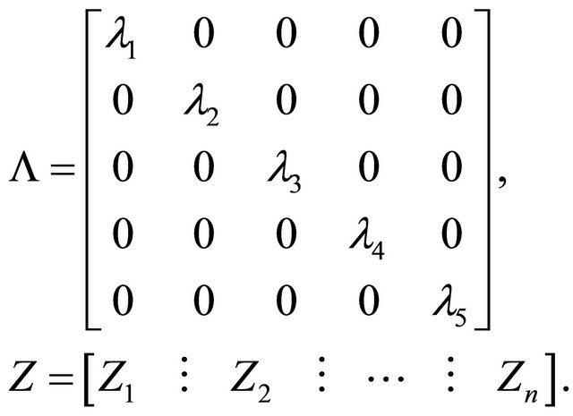
(1)
where  is a diagonal matrix of eigenvalues. Eigenvector robustness is a relatively recent area of exploration with the bulk of the existing related literature in the area of eigenstructure assignment and stability under parametric uncertainty; see [6] and [7]. Kato [8] considers perturbations in eigenspace and provides a functional relationship between eigenvalue perturbations (sufficiently small) and corresponding eigenvectors but this functional relationship requires the computation of a matrix inverse and definite integral. The following sections detail the study of achievable sets of eigenvectors which are associated with sets of uncertain matrices, examining special features in various matrix constructions. We focus on matrix constructions based on interval polynomials. We seek a new result which provides for a robustness measure on eigenvector variation over sets of matrices, but does not require matrix integration, extensive Monte Carlo and other sampling methods determine the set of achievable of eigenvectors. We will use
  to denote complex conjugation and
  to denote the transpose of x where x is a matrix or vector quantity.
2. Preliminaries
Before the major contributions of the paper are detialed, we introduce some needed concepts.
2.1. Interval Polynomials
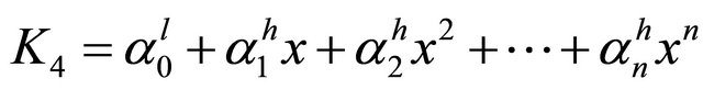
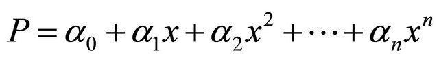
Our construction for this problem begins with a set of uncertain matrices generated from an interval polynomial with the following form:

The  parameters are interval parameters which make up an interval vector
 , where
We also define a center vector of the interval parameters,
For the specific numeric simulations and examples to follow in this paper, we choose . This allows nontrivial examples to be generated.
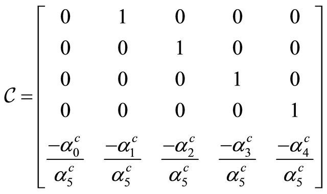
2.2. Companion Form Matrices
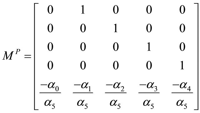
The companion form matrices are a standard construction associated with a polynomial equation. See [9] for detials. From the previously introduced interval polynomial, a standard construction yields the companion form matrix . For example with
  one obtains
2.3. Kharitonov Polynomials and Associated Companion Matrices
The Kharitonov polynomials are four specially constructed fixed polynomials associated with an interval polynomial which can be used to guarantee root stability results over the set of interval parameters using only the four functions. This celebrated result yields a test for stability in which the number of polynomials is fixed and does not depend on n. For example, we list the four Kharitonov polynomials for the interval polynomial structure of interest. The interested reader is referred to [10] for a more complete description.
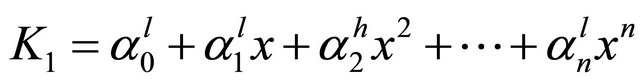
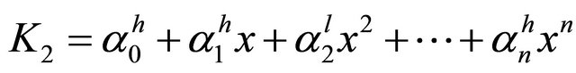
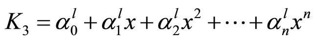
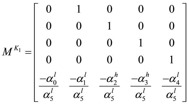
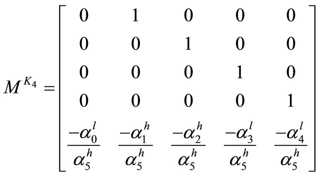
Also, for completeness, we illustrate the companion form of the four Kharitonov matrices.
Kharitonov matrix corresponding to .
.
Kharitonov matrix corresponding to .
.
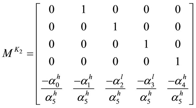
Kharitonov matrix corresponding to .
.
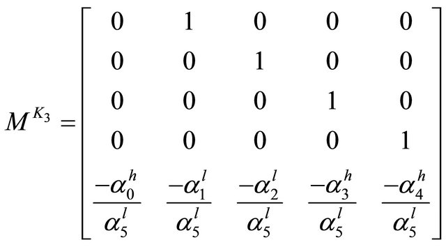
Kharitonov matrix corresponding to .
.
3. Eigenvector Containment Cones
Referring to (1), we can find  by solving for the roots of the characteristic equation of A. Our focus is on the eigenvector set, but it is obvious that the eigenvalue set is linked to the eigenvector set through Equation (1). We first need to introduce the construction of eigenvector paths between any two Kharitonov companion form matrices,
  and
and , where
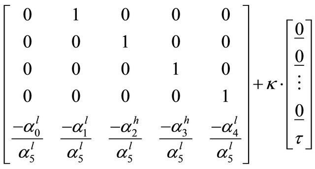
 . We construct these paths through a linear interpolation of the two Kharitonov matrices. We denote these paths as a collection of eigenvectors,
  where
where
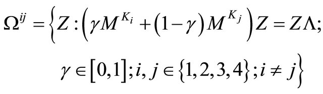 (2)
(2)
with
We wish to show that under certain constraints (later defined as having property ) a specific continuous eigenvalue path generated through an interval path of the interval polynomial corresponds to a unique eigenvector path. This will allow us to relate eigenvalue path bounds to eigenvector path bounds.
Proposition 1: Given a positive interval polynomial, P, and associated companion form matrix, A, with corresponding eigenvector matrix (V) and eigenvalue matrix ( ) containing distinct non-zero eigenvalues over the interval of P, any real or complex eigenvalue path has an associated unique real or complex eigenvector path.
Proof of Proposition 1:
We first introduce some machinery for the proof.
Implicit Function Theorem [11]: Let  be open and let
  be continuously differentiable. Let
  be such that
Then there is an open interval , such that
 , and there is a function
  which is continuously differentiable, such that
 , for all
 , and such that
 , for all
 .
.
We will use the matrix version of the Implicit Function Theorem where the matrix of function equations,  , is defined with the following conditions:
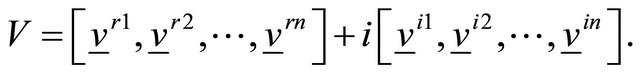
We also introduce a diagonalization procedure from Delchamps [12] to use in the formulation of constraint equations. Writing a complex  eigenvector,
  , as a function of two real vectors,
  and
and ,
,
we build an orthogonal eigenvector matrix,  , where

and . Here,
  is a diagonal matrix of eigenvalues of
  with imaginary eigenvalue pairs appearing as
  blocks with the real part on the diagonal and imaginary parts on the off-diagonal (positive imaginary part on the super-diagonal and negative imaginary part on the sub-diagonal). This is the same mapping as developed from the Schur factorization with well defined mapping P.
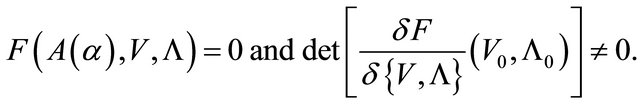
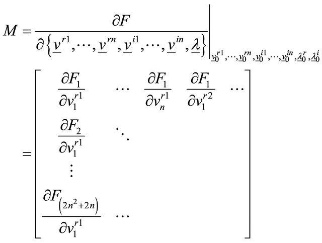
Given the Implicit Function Theorem, we construct a set of constraint equations from (1),
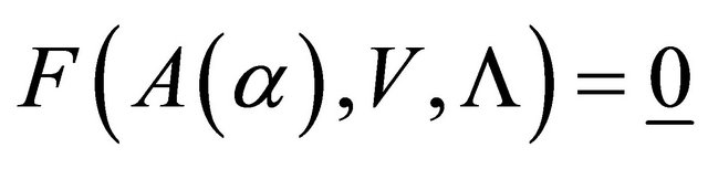
where
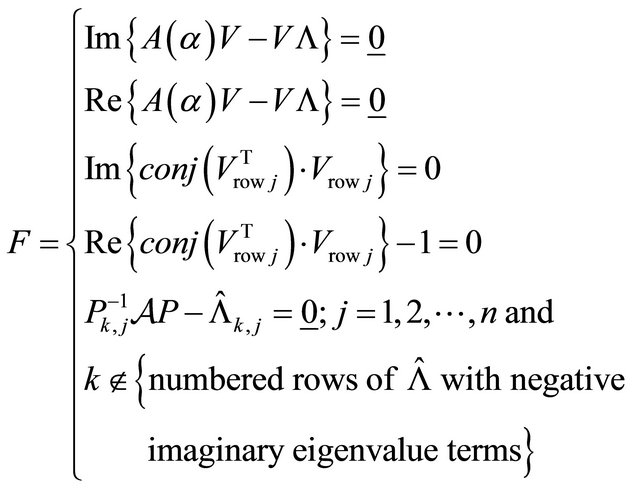
These constraint equations constrain the solution of eigenvectors such that 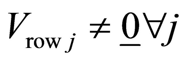 and constrain the form of complex eigenvalues of
  to complex conjugate pairs. The dimension of F is
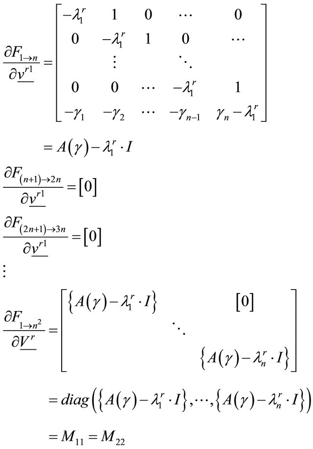
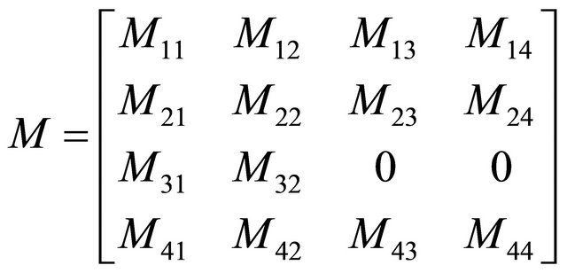
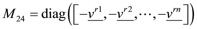
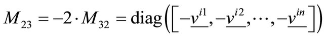
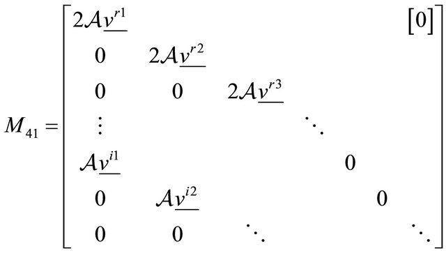
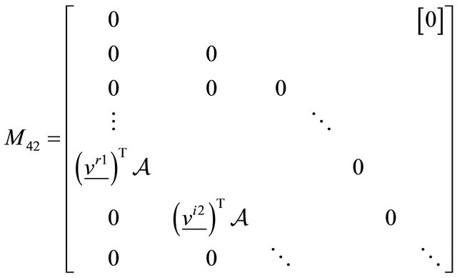
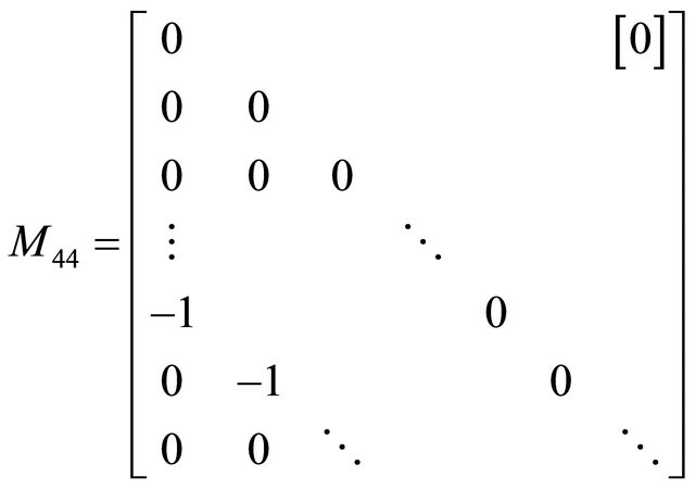
 . We write the partial derivative matrix M as follows,
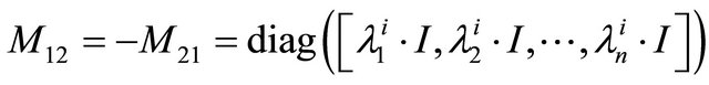
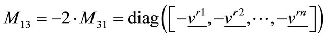
and construct the components
where  and
and  are block elements of
 . To complete
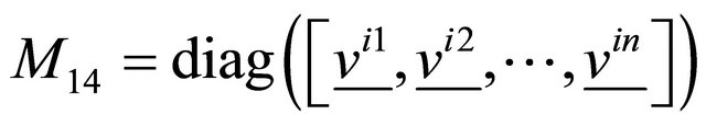
  we write
where

We seek the determinant of M. We define the determinant of M as a block matrix computation where 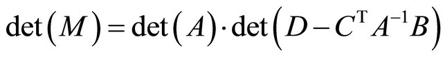 and
and
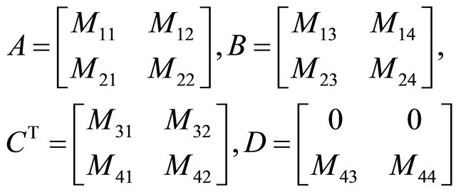
We take advantage of the diagonal structure of the sub-matrices of M to compute  and the determinants. Extensive matrix computation is required and is not included here, however the result shows
  under the conditions of distinct non-zero eigenvalues over the domain of eigenvalue space. The proposition is proved. We now define property
 .
.
Property : An interval matrix, A, with property
  is one having all eigenvalues of A distinct and non-zero over the interval parameter domain of the interval matrix.
This implies that a specific continuous eigenvalue path generated through an interval path of the interval polynomial corresponds to a single unique eigenvector path. We will attempt to utilize the Kharitonov companion form matrices to generate boundary points for these eigenvector paths. Once a boundary is defined, we can generate a containment eigenvector cone. A proposition is stated below.
Proposition 2: Given a positive interval polynomial, P, with property , the smallest normed cone containing the four eigenvectors along a single connected path associated with a single eigenvalue path and generated from the Kharitonov companion form matrices
  is a containment cone for the entire path of eigenvectors formed from the linear interpolation of matrices between any two
  and
and .
.
The vectors in the set  define a continuous path through n-dimensional space. Similarly, one could construct eigenvalue paths using the same interpolated matrices. These would be the corresponding eigenvalue paths where the
  eigenvalue path corresponds to the
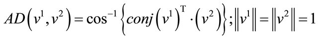
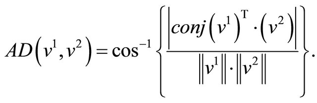
  eigenvector set. Assuming no two eigenvalue paths intersect, we can easily build isolated paths by solving (2). If any of the real eigenvalue paths intersect with the imaginary axis, two things will necessarily occur. The eigenvalue structure will change since two eigenvalues will become imaginary and a corresponding change in the eigenvector matrix will occur. This was found to introduce computational difficulty in tracking eigenvalue/ eigenvector pair paths due to the change in structure of the eigenvalue/eigenvector pairs. In an attempt to side step this computational difficulty, for some simulations, we restricted our cases of interest to those in which no eigenvalue paths cross the imaginary axis. We further restricted the polynomial parameter intervals to strictly positive intervals to ensure that the degree of P was unchanged over the parameter intervals. This will be discussed further in the sequel. Now we have defined the construction of the eigenvector paths, it remains to address the construction of the smallest containing cone for the eigenvectors of the four Kharitonov companion form matrices. We first need a metric for the size of a cone in n-dimensional space. We define an angular distance measure,
  , between any two normalized ndimensional vectors,
  and
and , which provides the basis of that metric.

Three methods were considered to find the containing cone for the four Kharitonov companion form matrix eigenvectors. These are detailed in the following sections.
3.1. Angle Bisector Method
The first approach we considered was to find the bisector of all two vector combinations of the four Kharitonov eigenvectors, determine the largest angular distance measure,  , between these six bisectors,
  , and their eigenvector pairs and construct a cone,
  , centered at the bisector
  corresponding to
  with the cone boundary defined by the following
The bisectors,  , for any pair of eigenvectors can be found be rescaling one of the vectors such that the projection of the other vector onto it is purely real. The eigenvectors in general are complex. In this way a real bisector can be found. Considering any two vectors
  and
and  we can find the bisector by first rescaling
 ,
,
then we can determine the bisector ,
,
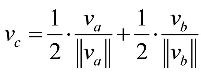
3.2. Optimized Centering Vector Method
With this method we construct a gradient based search method which seeks a “Centering” vector having the same angular distance measure from all four Kharitonov eigenvectors. Given a collection of i eigenvectors  Rn from
  we wish to solve the following max-min problem,
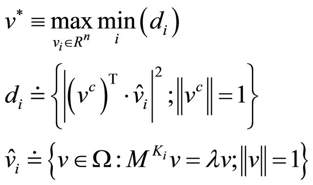
This optimization problem attempts to minimize the maximum angular distance measures between the optimal centering vector and all other Kharitonov eigenvectors. We seek to accomplish this with a gradient based algorithm which moves  “close” to
  in norm over a finite number of iterations. The algorithm is detailed below:
1) Initialize  at
at  and
and .
.
2) 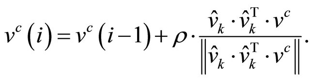
3) .
.
4) Find the  which satisfies
 .
.
5) .
.
6) Repeat step 2.
The algorithm does tend to converge to a normed cone if not a single vector since there does not necessarily exist a single vector solution, e.g. two or more Kharitonov eigenvectors are co-planar. A check of this result which yields a heuristic argument supporting its effectiveness is to measure  where
where  and
and
If 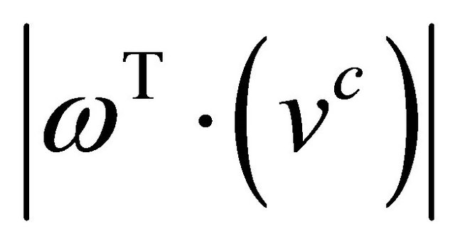 results in a quantity close to 1 then the two vectors are nearly aligned. This also yields credence to using eigenvectors generated from Kharitonov companion matrices as extremal eigenvectors.
3.3. First Order Perturbation Based Normed Cone Method
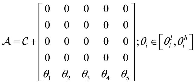
This method involves the application of a first order Taylor series approximation to the nominal companion form matrix defined earlier. This derives a sensitivity result for the uncertain parameters in the interval polynomial from which the companion form matrix was written. The derivation in this section follows from the matrix eigenvalue sensitivity results of Eisenstat and Ipsen [13]. Also see [14] for a similar companion matrix eigenvector perturbation construct. We define the interval companion matrix  with
with  as
as
With 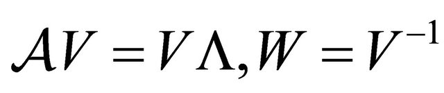 and
and 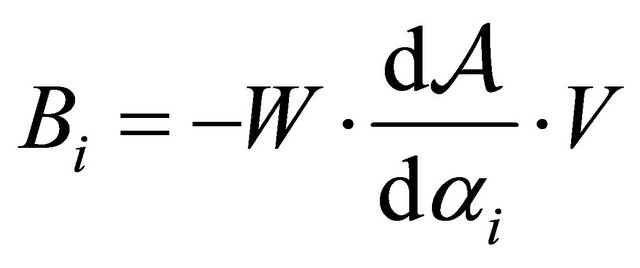 we can write the following
We can simplify the notation somewhat by writing
Then
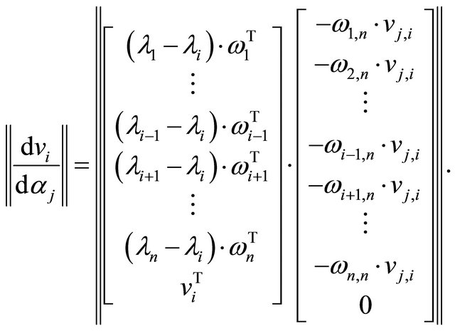
We can compute  by finding
  and solving the following,
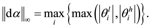
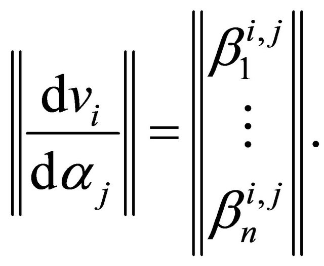
Now we can write the normed perturbation of ,
,  , as
, as
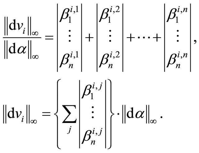
Similarly, we can write equations for all  to define the first order perturbation for any eigenvector in
 . Now that we have a vector representing a normed perturbation from the nominal
  we can build a normed cone with angular radius
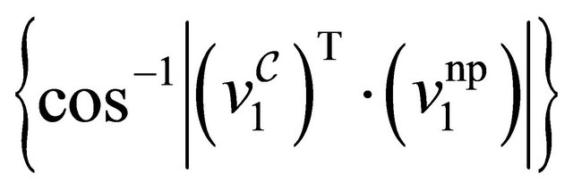 .
.
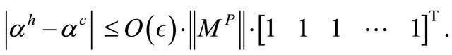
The derivation of the method of first order perturbations can be checked by comparing it to a known linear perturbation in the parameter space of . The error between the known linear perturbation eigenvector and that which is generated from the first order perturbation method should be proportional to the squared infinity norm of the perturbation vector. The following relation holds if the first order approximation is correct as
 ,
,
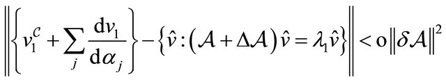
where
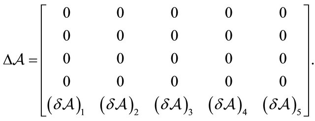
Through simulations, this was demonstrated to be true. We provide an example result based on the following matrix and perturbation configuration,
Using the configuration above, Figure 1 was generated. Note that the curves suggest increasing quadratic forms with respect to the perturbation scaling .
.
4. Results and Comparisons of Methods
First, we show an example of an interval companion matrix eigenvector continuous path construction using the four Kharitonov companion matrices as detailed in the beginning of the summary report. Since the example has dimension , we show a plot of the metric of inter-
Figure 1. Plots of the normed perturbation squared,  , and the scaled normed error between the known linear perturbation eigenvector and the eigenvector from the first order perturbation method.
est along the path. Only one eigenvector path is utilized although for the full extent of the methods described, all n eigenvector paths would need to be incorporated. The plot is shown in Figure 2. In this example, the position of the Kharitonov eigenvectors, every 2000-th iteration, yields a locally large value for the metric. This would allow for the use of the Kharitonov eigenvectors as the basis for finding a containment cone.
In Figure 3 we show an example of an interval companion matrix which, through the use of the metric along a continuous eigenvector path, has eigenvectors with a larger metric value than that at the Kharitonov eigenvectors. In this case the Kharitonov eigenvectors are not sufficient to define the path containment cone. This will be addressed as a restriction to the interval space which will be detailed in the following sections.
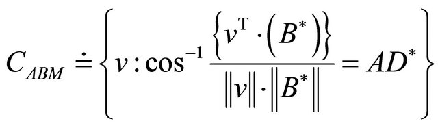
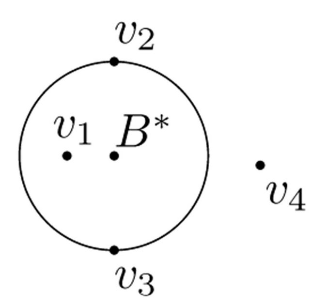
The first method does not guarantee containment of all four Kharitonov eigenvectors. This is shown graphically below. The four Kharitonov eigenvectors are scaled to project into the plane, Q, of the page and appear as points  in the plane. A cone is formed around
  which is shown as a circle in the cone cross-section in plane Q. By definition, the cone must contain at least two of the Kharitonov eigenvectors. Since the projection of the cone in plane Q, shown as the circle in the diagram, does not contain all the Kharitonov eigenvectors, the eigenvector continuous path cannot be contained by the circle. This implies that the cone is not a containment cone.
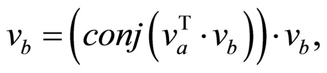
The second method is an iterative approach so taking the number of iterations out to infinity yields the following if the method converges to a single vector:
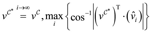
A normed cone can now also be constructed with an angular radius using the above formula. If the method does not converge, which could happen in the case of the non-existence of an equi-angularly distant centering vector, the method will converge in  steps to a normed ball centered at
  with radius
  containing a vector such that
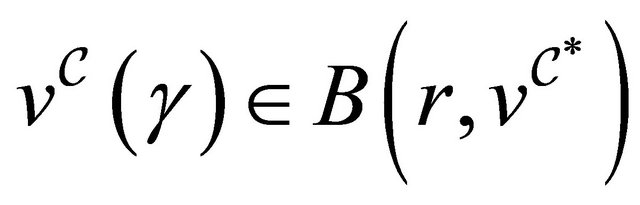
with  defined as
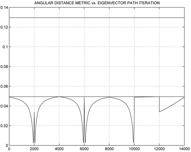
Figure 2. This figure shows an overlay of three curves. The first is AD* computed along a portion of one of the possible Ωij paths. The second and third curves are horizontal lines indicating AD* computed for the eigenvectors at the path boundaries. Path contained.
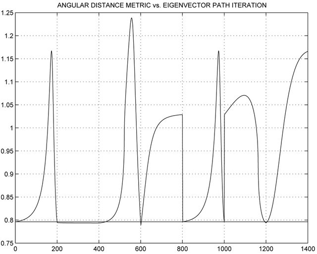
Figure 3. Overlay of AD* at path boundaries and over a portion of a possible Ωij path. Path not contained.
Numerical experience with the second method suggests it does yield convergence to a normed ball centered at the optimal centering vector within a finite number of steps. The normed ball also appears to be very close to the eigenvector derived from the nominal matrix . An example is shown in Figure 4.
The third method provides a large over-bound on the containment cone radius. This is due to the use of induced infinity norms on the perturbation matrices. The angular radius from the third method can be compared to the angular radius generated from the second method. In all example cases generated, the Taylor series approximation based normed cone has a larger angular radius than that produced from the second method. The third method is conservative. In all numerical examples ex-

Figure 4. Plot of normed distance between vi and vC for  using the iterative method of Section 3.2.
amined, the eigenvector path is contained in both cones when all three of the following events do not occur.
1) Somewhere along the path, two or more out of the n eigenvectors cross paths and the path tracking algorithm gets lost. This could be addressed by considering all paths when constructing the cone.
2) One or more eigenvalues associated with the eigenvectors cross the imaginary plane. This changes the structure of the eigenvectors and causes discontinuities in the path. The change in structure occurs because having real intervals in the parameter space forces imaginary eigenvalues to appear in pairs. One eigenvalue crossing the imaginary plane would induce two complex eigenvalues. In conjunction, a similar structure change occurs in the eigenvector set.
3) A zero crossing occurs in one or more dimensions of the parameter interval space. This also changes the structure of the eigenvector set.
All three events can be addressed such that they do not occur if the infinity norm of the perturbation is kept much smaller than the minimal element of the center vector,  , and the parameters are restricted to strictly positive intervals. With these conditions in all numerical examples examined, the path is always contained by the containment cone generated from either method two or three.
5. A Sufficient Condition for Containment Cones
A monotonic result can be shown for the angular distance metric of interest assuming a restriction to either all positive or all negative eigenvalues. This would then support a containment result based on a normed cone. The monotonic result comes from the vector projection property of the metric. The metric is monotonic in . An extension of the work of Kharitonov provides an extremal eigenvalue result that can be extended to the eigenvector space and hence, the metric.
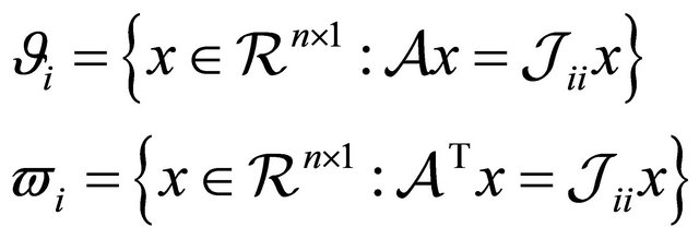
To complete this picture, one needs to show that the conditions discussed earlier to enable success of the simulations can be better defined. For that we utilize the contributions of [9] on perturbations of eigenvalues and eigenvectors. Given a matrix  as previously defined, with distinct eigenvalues, we can find the Jordan canonical form,
where the columns of  are the eigenvectors of
  and
and  a diagonal of the eigenvalues of
 . We further define
  as the normalized right and left hand eigenvectors respectively and
  such that
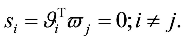
The right and left hand eigenvectors are defined as
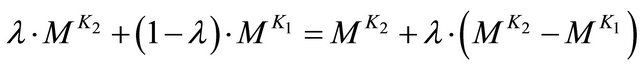
The parameter  is also the cosine of the angle between these eigenvectors. Recall the Kharitonov companion matrices have linear variation in elements of the last row only. This implies that the linear path between any two of these matrices can be written as
  with
with  since
since
 .
.
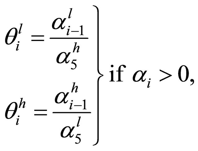
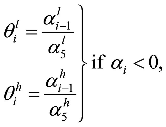
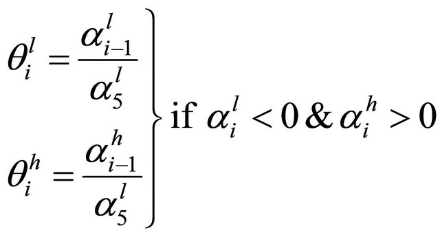
The following is an example using  and n = 5. The quantity
where 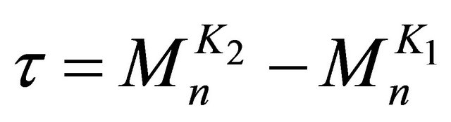 is a vector of constants dependent on the last rows of
  and
and . Now, incorporating the Jordan canonical form introduced above, from [9] we write
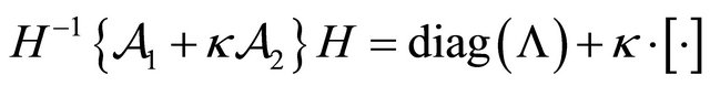
where
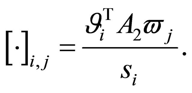
This implies from the Gerschgorim Theorems [9] that the distinct eigenvalues are located in disks with center
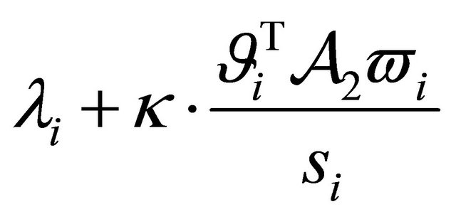 and radius
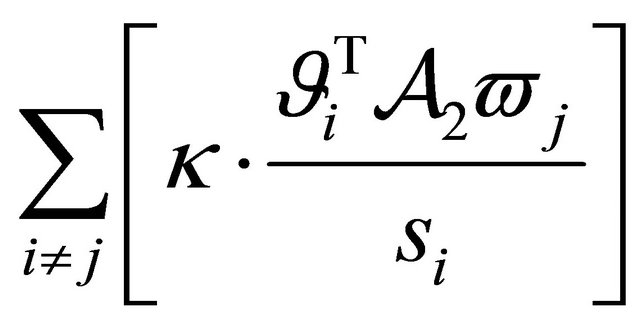 . A sufficient condition for the isolation of the eigenvalues,
  , over the path connecting the two Kharitonov companion matrices is shown in the following relation. For all
 ,
,
Given that the eigenvalue set at each Kharitonov companion matrix is sufficiently distributed, the above condition is satisfied and the eigenvalues will be isolated along the eigenvector pathways. We describe the family of polynomials with isolated roots such that the above condition is satisfied as having the property . We need one additional result from [10] chapter 9, namely the Stronger Root Version of the Edge Theorem. Given a family of polynomials
 , Barmish defines the root set of
  as the following
Stronger Root Version of the Edge Theorem [10]: Given a polytope of polynomials  with invariant degree, it follows that
We have, therefore, that the boundary of the root set or the extrema of the root set are contained within the edges of the family of polynomial polytopes. This result can be applied to the problem at hand by considering the eigenvalue set of the Kharitonov companion matrices as the root set of the family of Kharitonov polynomials. The edges of the family are the pathways between Kharitonov polynomials, and hence, Kharitonov companion matrices. This implies that the extremal eigenvalue set for the Kharitonov companion matrices lie along the edges or pathways between Kharitonov companion matrices. We can further say that the extremal eigenvalue sets are derived from the four Kharitonov companion matrices based on the Kharitonov Rectangle [10] construction. Now we complete this section with an illustrative example.
Numerical Example of the Sufficiency Condition for the Isolation of Eigenvalues
Given that we can write the linear path between any two Kharitonov companion form matrices  and
and  of dimension
  with
with  as
as
we build a constraint with  and
and  having the following characteristic polynomials
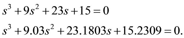
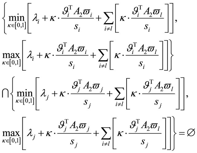
Now computing the constraint quantities we find that the three ranges of eigenvalues for  and
and  respectively are

The intersection of these three ranges is the empty set. Therefore,  and
and  represent two matrices with eigenvalues that do not intersect along the path between them. This same test could be applied to the six combinations of Kharitonov companion form matrices to test whether all eigenvalue ranges are sufficiently distributed over all paths between matrices.
6. Proof of Proposition 2
The proof follows primarily from the results of the previous section, the specialized structure of the metric of interest and the eigenvectors generated from the Kharotonov companion matrices. For this proof we need to show that the four Kharitonov companion matrices generate extremal eigenvector sets in terms of the metric of interest. This follows from having extremal eigenvalue sets since the eigenvectors are in the form
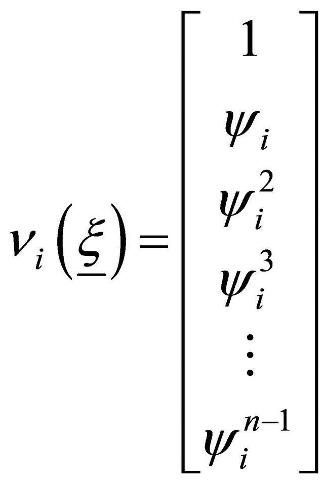
and extremal eigenvalue sets generate extremal quantities
 with all real half-plane roots. We have the additional property of half-plane roots since the family of polynomials of interest are restricted to positive intervals. Now with extremal eigenvalue sets generated from the four Kharitonov companion matrices, we see that these sets lead to the extremal eigenvector metric
or
It follows that the angular distance of a given eigenvector, constructed from the companion form family of polynomials, P, from a pre-defined centering vector has a normed bound less than the angular distance of at least one eigenvector constructed from the companion form of the four Kharitonov matrices. Furthermore, this implies a minimum norm containment cone can be constructed around the eigenvectors constructed from the companion form of the four Kharitonov matrices. This set of eigenvectors contains all eigenvectors, and hence any path of eigenvectors, constructed from the companion form family of polynomials, P. This completes the proof.
7. Summary and Discussion
In this paper we have developed some tools and a robustness result methodology through which may build a containment cone for the eigenvector space of a companion form matrix associated with an interval polynomial. This method involved strong use of the well know Kharitonov polynomials which allowed for a computationally inexpensive technique for a broad class of interval polynomials. It is true that computational accuracy is limited when converting from a polynoimial form to a companion form. Edelman and Murakami [15] address this issue objectively by suggesting that one bound the variation in polynomial parameter space by a scaling of the norm of the associated companion matrix, i.e. given
then one should require
where  signifies a small multiple of machine precision. This clearly restricts the utility of the results of this paper however it invites a challenge to consider specific polynomial forms which may ease this requirement. That is the subject of future work.
REFERENCES
- R. Smith, “Eigenvalue Perturbation Models for Robust Control,” IEEE Transactions on Automatic Control, Vol. 40, No. 6, 1995, pp. 1063-1066. doi:10.1109/9.388684
- T. Alt and F. Jabbari, “Robustness Bounds for Linear Systems under Uncertainty: Eigenvalues Inside a Wedge,” Journal of Guidance, Control, and Dynamics, Vol. 16, No. 4, 1993, pp. 695-701. doi:10.2514/3.21069
- S. Wang, “Robust Schur Stability and Eigenvectors of Uncertain Matrices,” Proceedings of the American Control Conference, Vol. 5, 1997, pp. 3449-3454.
- P. Michelberger, P. Varlaki, A. Keresztes and J. Bokor, “Design of Active Suspension System for Road Vehicles: An Eigenstructure Assignment Approach,” Proceedings of the 23rd Fédération Internationale des Sociétés d’Ingénieurs des Techniques de l’Automobile (FISITA) World Automotive Congress, Torino, 1990, pp. 213-218.
- D. Hinrichson and A. J. Pritchard, “Mathematical Systems Theory I: Modelling, State Space Analysis, Stability and Robustness,” Springer, Berlin, 2005.
- S.-G. Wang and S. Lin, “Eigenvectors and Robust Stability of Uncertain Matrices,” International Journal of Control and Intelligent Systems, Vol. 30, No. 3, 2002, pp. 126-133.
- R. Patton and J. Chen, “On Eigenstructure Assignment for Robust Fault Diagnosis,” International Journal of Robust and Nonlinear Control, Vol. 10, No. 14, 2000, pp. 1193-1208. doi:10.1002/1099-1239(20001215)10:14<1193::AID-RNC523>3.0.CO;2-R
- T. Kato, “Perturbation Theory for Linear Operators,” Springer-Verlag, New York, 1966. doi:10.1007/978-3-642-53393-8
- J. H. Wilkinson, “The Algebraic Eigenvalue Problem,” Oxford University Press, Oxford, 1965.
- B. Barmish, “New Tools for Robustness of Linear Systems,” Macmillan Publishing Company, New York, 1994.
- C. Goffman, “Calculus of Several Variables,” Harper and Row Publishers, New York, 1965.
- D. Delchamps, “State Space and Input-Output Linear Systems,” Springer-Verlag, New York, 1988. doi:10.1007/978-1-4612-3816-4
- S. Eisenstat and I. Ipsen, “Three Absolute Perturbation Bounds for Matrix Eigenvalues Imply Relative Bounds,” SIAM Journal on Matrix Analysis and Applications, Vol. 20, No. 1, 1998, pp. 149-158. doi:10.1137/S0895479897323282
- F. Bazán, “Matrix Polynomials with Partially Prescribed Eigenstructure: Eigenvalue Sensitivity and Condition Estimation,” Computational and Applied Mathematics, Vol. 24, No. 3, 2005, pp. 365-392. doi:10.1590/S0101-82052005000300003
- A. Edelman and H. Murakami, “Polynomial Roots From Companion Matrix Eigenvalues,” Mathematics of Computation, Vol. 64, No. 210, 1995, pp. 763-776. doi:10.1090/S0025-5718-1995-1262279-2