American Journal of Operations Research
Vol.3 No.1A(2013), Article ID:27550,14 pages DOI:10.4236/ajor.2013.31A016
Recent Developments in Monitoring of Complex Population Systems
1Institute of Mathematics and Informatics, Szent István University, Godollo, Hungary
2Department of Mathematics, University of Almería, Almería, Spain
Email: *Varga.Zoltan@gek.szie.hu, mgamez@ual.es, milopez@ual.es
Received November 29, 2012; revised December 30, 2012; accepted January 15, 2013
Keywords: Ecological Chain; Fishery with Reserve Area; Stable Coexistence; Ecosystem Monitoring; Verticum-Type System; Nonlinear System; Observer Design
ABSTRACT
The paper is an update of two earlier review papers concerning the application of the methodology of mathematical systems theory to population ecology, a research line initiated two decades ago. At the beginning the research was concentrated on basic qualitative properties of ecological models, such as observability and controllability. Observability is closely related to the monitoring problem of ecosystems, while controllability concerns both sustainable harvesting of population systems and equilibrium control of such systems, which is a major concern of conservation biology. For population system, observability means that, e.g. from partial observation of the system (observing only certain indicator species), in principle the whole state process can be recovered. Recently, for different ecosystems, the so-called observer systems (or state estimators) have been constructed that enable us to effectively estimate the whole state process from the observation. This technique offers an efficient methodology for monitoring of complex ecosystems (including spatially and stage-structured population systems). In this way, from the observation of a few indicator species the state of the whole complex system can be monitored, in particular certain abiotic effects such as environmental contamination can be identified. In this review, with simple and transparent examples, three topics illustrate the recent developments in monitoring methodology of ecological systems: stock estimation of a fish population with reserve area; and observer construction for two vertically structured population systems (verticum-type systems): a four-level ecological chain and a stage-structured fishery model with reserve area.
1. Introduction and Historical Overview
Mathematical Systems Theory (MST) looks back on several decades of history. In engineering practice, it is a typical situation that an object (e.g. a machine or electronic circuit) is controlled by a human intervention to influence the state of the object, or observing a transform of the state the task is to recover the state process of the object. The corresponding concepts of controllability, observability and the related state space model played an important role in the development of MST. The first comprehensive monograph of this discipline, dealing only with linear systems, was [1], a more recent reference is [2]. Generalizations of controllability and observability theory to nonlinear systems can be found in [3]. Following a successful development of MST for engineering purpose, as a new research line, in [4,5] the application MST to the study of population systems was proposed.
For population system, observability means that, from partial observation of the system, in principle, the whole state process can be recovered. Recently, for different ecosystems, the so-called observer systems (or state estimators) have been constructed that enables us to effectively estimate the whole state process from the observation. This technique offers an efficient methodology for monitoring of complex ecosystems (including spatially and stage-structured population systems). In this way, from the observation of a few indicator species the state of the whole complex system can be monitored, in particular certain abiotic effects such as environmental contamination may be identified.
In fact, the systems-theoretical study of the considered nonlinear frequency-dependent population models required the generalization of general sufficient conditions for controllability and observability to the case of nonlinear systems with invariant manifold (see [4,5]). These results have been applied to a control-theoretical model of artificial selection, phenotypic observation of genetic processes and evolutionary game dynamics, as well as to systems-theoretical models of reaction kinetics, see [6- 15].
Later on, the methodology of MST was used for monitoring of different population systems: observability and system inversion were investigated in density-dependent models of population ecology, ranging from Lotka-Volterra-type ([16-18]) and non Lotka-Volterratype population systems to monitoring of environmental change in a complex ecosystem ([19]). In particular, in [20] the optimal control software developed in [21] and [22], was also used for equilibrium control of a trophic chain. In [23] a new nonlinear system inversion method was applied for the reconstruction of time-dependent abiotic environmental changes, from the observation of certain indicator species. Furthermore, both monitoring and control were studied in a systems-theoretical model of radiotherapy in [24], while in [25-27] tools of MST were applied to biological pest control. Most of these topics and results have been reviewed in the survey papers [28] and [29].
In the present survey we report on recent developments in the methodology and application areas of monitoring in complex ecological systems. Although the presented methodology can be applied for the monitoring of large, but appropriately structured complex population systems, for the sake of simplicity and transparency we illustrate the procedures on observation systems of low dimensions. A particular attention is paid to recent results concerning the so-called verticum-type observation systems. The linear version of such systems have been introduced for modelling certain industrial systems and studied for controllability and observability in [30-38]. Verticum-type systems are composed from several “subsystems” connected sequentially in a particular way: a part of the state variables of each “subsystem” also appears in the next “subsystem” as an “exogenous variable” which can be also interpreted as a control generated by an “exosystem”. Therefore, these “subsystems” are not observation systems, but formally can be considered as controlobservation systems. The problem of observability of such systems can be reduced to rank conditions on the “subsystems”, which is a kind of decoupling of a complex system into simpler parts. Since most dynamic models of population biology are nonlinear, for the application in this field, it was necessary to extend the basic concepts and theorems of the theory of linear verticumtype systems to the nonlinear case, which has been done recently in [19,39-41].
The paper is organized as follows. In Section 2, based on [42], following a necessary stability analysis according to [43], the stock estimation of a fish population with reserved area is presented, using an appropriate observer design. In Section 3 results from [40] are recalled concerning the monitoring of ecological interaction chains of the type resource-producer-primary user-secondary consumer. The dynamic behaviour of these four-level chains is modelled by a system of differential equations, the linearization of which is a verticum-type system. Section 4 is devoted to the general concept of a nonlinear verticum-type observation system and the corresponding general sufficient condition of observability obtained in [41]. As an application, observer design is also presented for a stage-structured population, decomposing the state estimation according to the verticum structure. In Section 5 further possible application fields of the presented monitoring methodology are summarized. Finally, in the Appendix the theoretical background necessary for the monitoring of nonlinear verticum-type systems is recalled.
2. Stock Estimation of a Fish Population with Reserved Area
For the basic model of this section, from [43] we recall the dynamics of a fish population moving between two areas, the first, an unreserved one where fishing is allowed, and the second, a reserved one where fishing is prohibited. At time t, let x1(t) and x2(t) be the respective biomass densities of the same fish population inside the unreserved and reserved areas, respectively. Assume that the fish subpopulation of the unreserved area migrates into the reserved area at a rate m12, and there is also an inverse migration at rate m21. Let E be a constant fishing effort applied for harvesting in the unreserved area and let us assume that in each area the growth of the fish population follows a logistic model. The dynamics of the fish subpopulations in unreserved and reserved areas are then assumed to be governed by the following system of differential Equations (1) and (2):
 (1)
(1)
 , (2)
, (2)
where r1 and r2 are the intrinsic growth rates of the corresponding subpopulations, K1 and K2 are the carrying capacities for the fish species in the unreserved and reserved areas, respectively; q is the catchability coefficient in the unreserved area. All parameters r1, r2, q, m12, m21, E, K1 and K2 are positive constants.
In [43], it was checked that for a unique positive equilibrium  of the dynamic model (1)-(2) the following set of inequalities are sufficient:
 (3a)
(3a)
 (3b)
(3b)
 (3c)
(3c)
Furthermore, the Lyapunov function

also implies asymptotic stability of equilibrium  for system (1)-(2), globally with respect to the positive orthant of
 . Throughout the section we shall suppose conditions (3a)-(3c) to guarantee the stable coexistence of the system applying a constant reference fishing effort.
2.1. Observability of the Model
From [3], we recall the basic concept of local observability of nonlinear systems and a sufficient condition for a system to have this property, in order to apply it to the considered model and in order to be used in the following sections.
Let

and consider observation system
 (4)
(4)
 , (5)
, (5)
where function (5) defines the transform of the state, observed instead of the state itself.
Definition 2.1. System (4)-(5) is called locally observable at  on
on , if for any solutions
  of (4) defined on
 , initially close enough to
 ,
,
 .
.
Linearizing (4)-(5) around , we get
 .
.
Theorem 2.1. ([3]) 
system (4)-(5) is locally observable at  on
on .
.
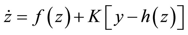
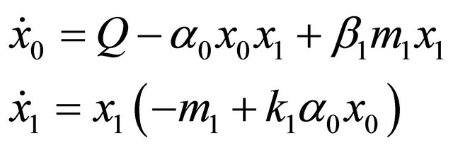
Now, let us consider the problem of stock estimation in the reserve area on the basis of the biomass harvested in the free area. (For technical reason its difference from the equilibrium value is supposed to be observed.) To this end, in addition to dynamics (1)-(2) we introduce an observation equation
 (6)
(6)
representing the observation of the biomass harvested in the free fishing area. Then linearizing observation system (1)-(2), (6), we get the Jacobian of the right-hand side of (1)-(2)
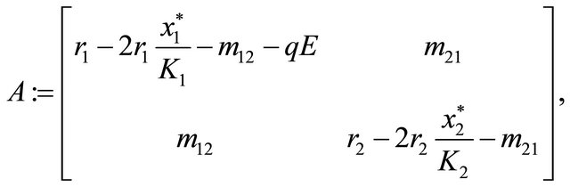
and the observation matrix
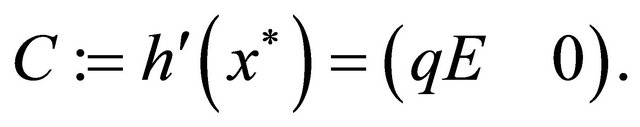
Now, for the linearized system we obviously have 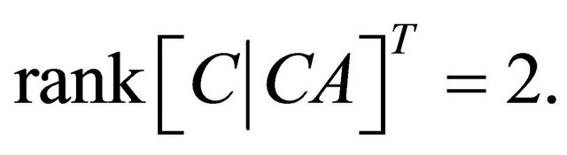 Hence, Theorem 2.1 implies local observability of the system near the equilibrium. In other words, in principle the whole system state (in particular the stock of the species in the reserve area) as function of time can be uniquely recovered, observing the biomass harvested per unit time. In the following illustrative example we will see how the state of the system (and hence the total stock) can be effectively calculated from the catch realized in the fishing area, applying the methodology of [44] that we will recall next.
2.2. Observer System
Recently, for different ecosystems, the so-called observer system (or state estimators) have been constructed that enables us to effectively estimate the whole state process from the observation. Here we remind the methodology that will be used in this subsection and in the following sections. Consider again observation system (4)-(5)
 .
.
Definition 2.2. Given , system
 (7)
(7)
is called a local (exponential) observer for system (4)-(5) at , if for the composite system (4)-(5), (7) we have 1)
 2) there exists a neighbourhood
  of
of  such that
 (exponentially).
Theorem 2.2. ([44]) Suppose equilibrium  of system (4) is Lyapunov stable, and there exists nxn matrix
  such that
  is stable. Then system
 (8)
(8)
is a local exponential observer for observation system (4)-(5).
Example 2.1. For a possible comparison, in this numerical example we use the same parameters as [45]:
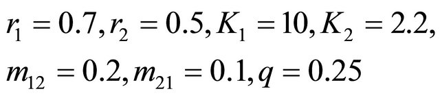
and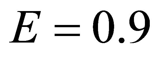 .
.
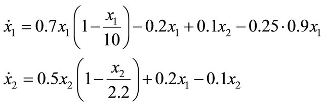 (9)
(9)
Now the positive equilibrium is , and with
matrix  is Hurwitz; therefore by Theorem 2.2 we have the following observer system
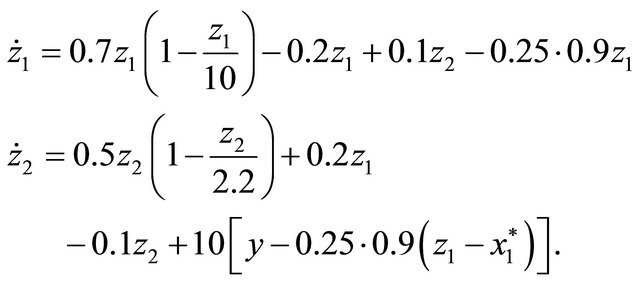 (10)
(10)
If we take an initial condition  for system (9), and similarly, we consider another nearby initial condition,
  for the observer system (10), then the corresponding solution
  of the observer tends to the solution
 ![]() of the original system, as shown in Figure 1. We note that in this particular case the convergence is much faster than that of the observer constructed in [45].
of the original system, as shown in Figure 1. We note that in this particular case the convergence is much faster than that of the observer constructed in [45].
3. Monitoring of a Four-Level Ecological Chain
As a modification of the well-known three-level trophic chain consisting of resource-producer-primary consumer studied in [46], we consider the following four-level ecological interaction chain:
level 0: a resource;
level 1: the producer is a plant, supposed to die out without the resource, and the positive effect of the latter is proportional to the quantity of the resource present in the system;
level 2: the primary user (instead of consumer), i.e. a commensalist animal, making use of the plant as part of its habitat without harming it (e.g. an insect species hosted by the plant), displaying a logistic dynamics in absence of the plant and the secondary consumer;
level 3: the secondary consumer is a monophagous predator of the primary user (e.g. an insectivorous singing bird species), with intraspecific competition.
(For more details on the role of commensalism in ecological communities, we supposed between the producer and the primary user, see e.g. [47]).
For a dynamical model let  be the time-dependent quantity, with a constant supply
  of the resource pre-

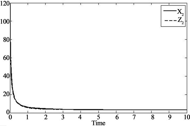
Figure 1. Solution of observer (10), approaching the solution of system (9).
sent in the system,  and
and  the time-varying population size (biomass or density) of the producer, the primary user and the secondary consumer, respectively. Assume that a unit of biomass of the plant consumes the resource at velocity
 ; however, it increases the biomass of the plant at rate
 . The relative rate of increase in biomass of the primary user, due to the presence of the plant is
 . While the plant population is supposed to die out exponentially in the absence of the resource, with Malthus parameter
 , the primary user displays a logistic growth with Malthus parameter
  and is limited by a carrying capacity
 . Furthermore, the secondary consumer would die out at rate
 , without the presence of the primary user, and there is an intraspecific competition among predators with rate
 . We will consider a partially closed system, where the dead plants may be recycled into nutrient resource with rate
 . Then with parameters
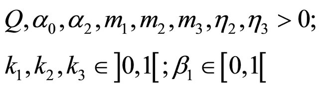 we have the following dynamic model for the considered interaction chain:
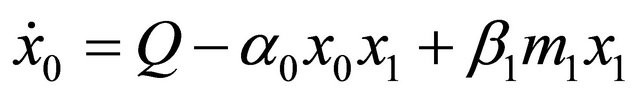 (11)
(11)
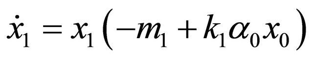 (12)
(12)
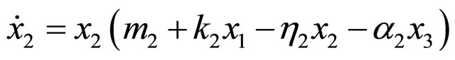 (13)
(13)
 (14)
(14)
Theorem 3.1. ([40]) Let us suppose that for given biological parameters, the resource supply is high enough,
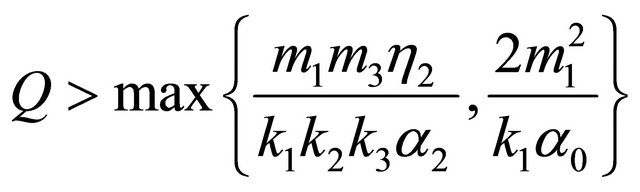 . (15)
Then, both the open  and the partially closed
  ecological chains stably coexist in the sense there exists a positive equilibrium
  of system calculated in [40], which is asymptotically stable.
Remark 3.1. The conditions of Theorem 3.1 can also be formulated conversely: Given a resource supply Q, biological parameters satisfying condition (15) imply the stable coexistence of the considered ecological chain.
3.1. Observability of the Ecological Chain
Let us consider now the following two auxiliary 2-dimension systems
 (16)
(16)
and
 . (17)
In ecological terms (16) is a subsystem of the original chain (11)-(14), while in (17) the positive effect of the plant on the animal species 2 appears with the equilibrium value  of the plant. We note that by setting
  (i.e. considering the original system without commensalisms), the original ecological chain is split up into two components without interaction.
Remark 3.2. The biological interpretation of system (17) is the following: Suppose that system (11)-(14) is in equilibrium, and the two animal species, by an external disturbance, deviate from their equilibrium densities. Then the resource-primary consumer subsystem can maintain its equilibrium, and the predator-prey subsystem will be governed by system (17).
Continuing the study of systems (16) and (17), we can easily check that they have respective equilibria  and
and . For system (16) with notation
 , let us consider observation function
 . (18)
This means that the deviation of the resource from its equilibrium value is observed. In order to check local observability, we calculate the linearization of system (16) at equilibrium :
:
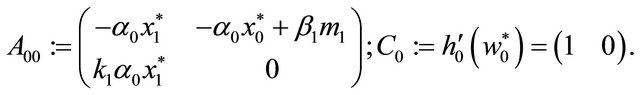 (19)
(19)
Hence we easily calculate
 provided
 . From the classical sufficient condition for the local observability of nonlinear systems, [3], we obtain local observability of system (16) near the equilibrium, with observation (18).
Similarly, suppose that in system (17) the deviation of the density of the prey from its equilibrium value is observed, i.e., with notation  we consider the observation function
 . (20)
The linearization of system (17) at equilibrium  is
is
 . (21)
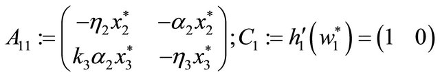
Checking again the rank condition, by  we get
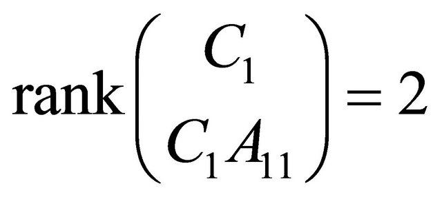 implying local observability of system (17)-(20) near
 . Now, let us observe that with definition
 system matrix
 together with observation matrix

define a verticum-type linear observation system in the sense defined in the Appendix. Applying Theorem A.2 of the Appendix, we obtain that the linear observation system
 (22)
(22)
 (23)
(23)
is observable. Since  is just the Jacobian of the righthand side of system (11)-(14), therefore (22) is just the linearization of system (11)-(14). Furthermore, (23) is the linearization of observation function
 (24)
(24)
which can be associated with system (11)-(14). Finally, applying again the classical rank condition of [3], we can summarize the reasoning of this subsection in the following theorem.
Theorem 3.2. Let us suppose that ecological chain (11)-(14) is partially closed .Then with observation function (24), system (11)-(14) is locally observable near equilibrium
  calculated in [40].
3.2. Construction of an Observer System
Following the procedure of [44], let us first determine conditions for the construction of observers for systems (16) and (17), with respective observation functions (18) and (20).
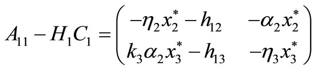
For matrices  and
and , figuring in (19), we have to find a matrix
  such that
is a Hurwitz matrix, i.e. all roots of the characteristic polynomial  of matrix
  have real negative parts. It is easy to check that the latter condition is satisfied if and only if the following inequalities hold:
 (25)
(25)
 . (26)
Simple sufficient conditions for (25) and (26) are  and
and , respectively. By the Theorem of [44], the observer for system (16) with observation function (18) can be determined.
Similarly, for matrices  and
and , figuring in (21), we need to find a matrix
  such that all roots of the characteristic polynomial
  of matrix
have real negative parts. Now a straightforward checking shows that the latter condition is satisfied if and only if  satisfy the following inequalities:
 (27)
(27)
 (28)
(28)
Similarly to the previous case, in order to satisfy conditions (27) and (28), it is sufficient to set  and
and , and again by the Theorem of [44], the observer for system (17) with observation function (20) can be determined.
Finally, based on the above reasoning, it will be easy to prove the following result:
Theorem 3.3. ([40]) Given
 with
with  and
and , and function
  defined as the right-hand side of system (11)-(14), system
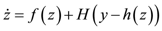
is a local exponential observer for system (11)-(14) with observation equation , where
  is defined in (24).
Example 3.1. We consider the following system
 (29)
(29)
System (29) has a positive equilibrium  , which is asymptotically stable, because conditions of Theorem 3.1 are satisfied. In Figure 2 it can be seen how, e.g. from initial condition
  near the equilibrium, the solution
 ![]() of system (29) tends to this positive equilibrium, see Figure 2.
of system (29) tends to this positive equilibrium, see Figure 2.
Consider now system (29) with observation
 .
.

Figure 2. Solution of system (29) with initial condition .
.
Since matrix
 satisfies the conditions of Theorem 3.3, we can construct the following observer
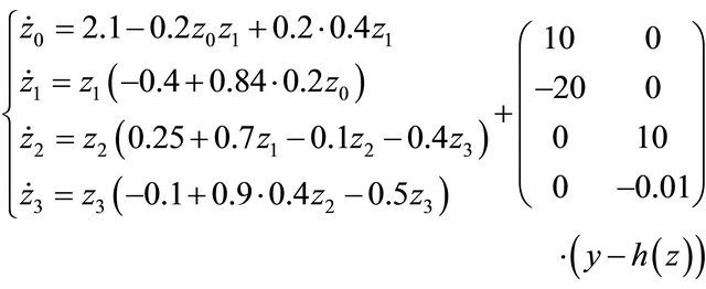 (30)
(30)
Solving (30) with initial condition  near the equilibrium, we can check how this solution tends to recover the corresponding solution of system (29), see Figure 3.
4. A Stage-Structured Fishery Model with Reserve Area
Let us consider a modification of the stage-structured fishery model of [45], supposing that there is reserve area where fishing is not allowed. In what follows, the first index of the biomass density  will indicate the area:
 ![]() for the reserve and
for the reserve and  for the free area; the second index will refer to the development stage:
  for the pre-recruits, i.e. the eggs, larvae and the juveniles together, and
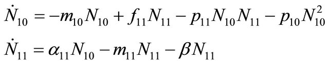
  the exploited stage of the population. The dynamics of the system is modeled by the following autonomous system of differential equations
 (31a)
(31a)

Figure 3. Solutions of systems (29) and (30) with the respective initial conditions  and
and .
.
 (31b)
(31b)
 (31c)
(31c)
 (31d)
(31d)
where
 natural mortality rate of class
 ![]() ,
,
 linear aging coefficient in areas
 juvenile competition parameter in areas
 fecundity rate of adult fish in areas
 predation rate of class 1 on class 0 in areas
 catchability coefficient of class 1 in the unreserved area,
 migration rate of the second class from reserved area to unreserved area,
 constant fishing effort.
From [41] we know that if
 (32)
(32)
system (31) has a unique positive equilibrium , which is asymptotically stable under conditions
 and
and  (33)
(33)
Remark 4.1. Since asymptotic stability implies Lyapunov stability, in the next section we can apply Theorem A.3 of the Appendix to the corresponding nonlinear verticum-type observation system.
4.1. Observability of the Model
Let  with
with ,
,  and we consider the observation function
  defined by
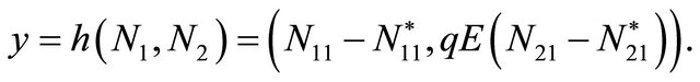 (34)
(34)
Now the observability of observation system (31)-(34) will be analyzed using the results of the Appendix. Consider systems
 (35)
(35)
and
 . (36)
Given observation
 (37)
(37)
we calculate its linearization
It is easy to check that , where
  is the linearization of (35), therefore by Theorem A.1 of the Appendix we can guarantee local observability of system (35)-(37).
Analogously, for observation
 (38)
(38)
of system (36) calculate
Again we have  , where
  is the linearization of (36), therefore from Theorem A.1 of the Appendix we have local observability of system (36)- (38). Since under the appropriate conditions equilibrium
  is asymptotically stable and hence also Lyapunov stable, applying Theorem A.3 we obtain Theorem 4.1. Suppose that conditions (32) and (33) hold. Then observation system (31)-(34) is locally observable near the asymptotically stable equilibrium.
4.2. Construction of an Observer System
Given the observation system (35)-(37), using the corresponding observer design of [44], it is sufficient to find a matrix  such that
  is Hurwitz. It is easy to check that with
  ,
,
is appropriate.
Analogously, for observation systems (36)-(38), with ,
,
 ,
,
 is Hurwitz, guaranteeing the construction of the observer system.
From these results, for

we can check that  is Hurwitz, which allows the construction of an observer for system (31)-(34) moreover, this observer is composed of the observers constructed for the two subsystems.
Example 4.1. Consider the following model parameters of [48]:

To construct the observer system for (35)-(37) we can take
 .
.
Then the observer system is
 (39)
(39)
Considering  as initial value for the system (35), and
  for the observer (39), in Figure 4 we can see how the solution of the observer system approaches the solution of the original system.
To construct the observer of system (36)-(38) take
Then the observer system is
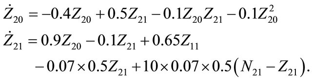 (40)
(40)
If we consider  as initial value for system (36), and
  for the observer (40)we obtain the result plotted in Figure 5.
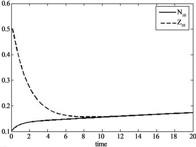

Figure 4. Solution of the observer (39) approaching the solution of the original system (35).
Now the observer for system (31)-(34) can be simply composed from the single observers (39) and (40). In Figure 6 we can see how the solution of the observer (39)-(40) with initial value , estimates the solution of system (31) with initial value
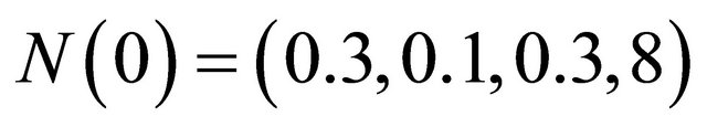 .
.
5. Discussion and Outlook
Observation problems arise in many fields of human activity, when state of an object can be characterized by several numbers (i.e. by a state vector), and it is impossible or too expensive to measure all state variables. Then
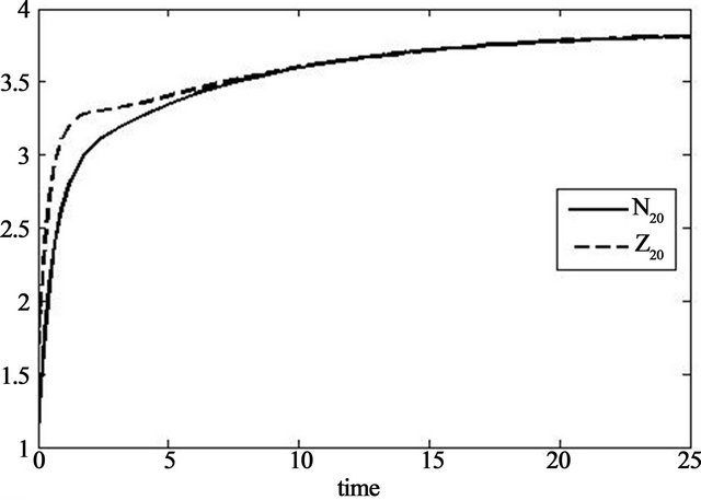
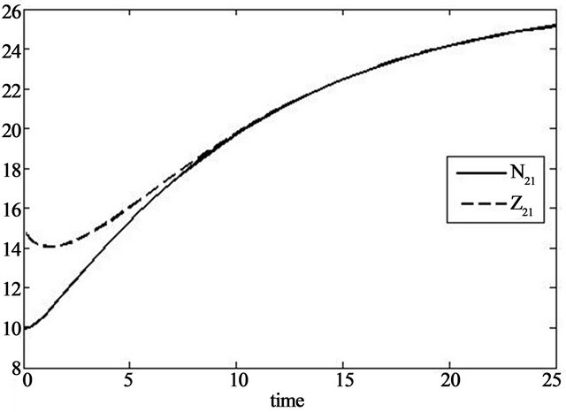
Figure 5. Solution of the observer (40) approaching the solution of the original system (36).
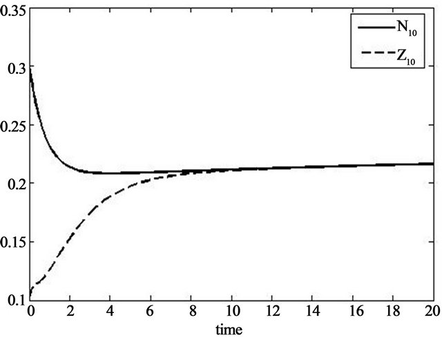
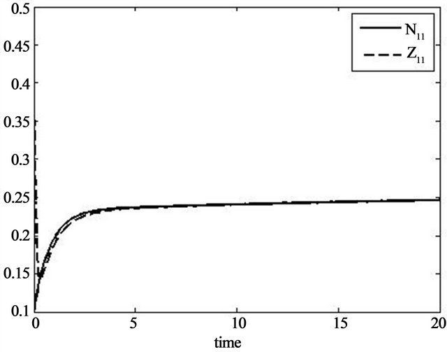


Figure 6. Solution of the observers (39) and (40) approaching the solution of the original system (31) by coordinates.
we may want to recover the whole state vector. In a static situation this is clearly impossible, since projection is not invertible. However, in dynamic situation the concepts of observability and observer design of Mathematical Systems Theory turned out to be efficient tools for monitoring of ecological systems, as well. We presented some recent developments in concrete applications to population systems. These systems are not only simple sets of populations, but each of them has a particular structure. In the first case (Section 2) a single species has a spatially structured habitat (with a reserve area, where observation of density by harvesting is not allowed). In the other two cases, verticum-type, i.e. vertically organized dynamic population systems (ecological chains in Section 3, and stage structure of a single species in Section 4), for monitoring purpose “decoupled” observer design may be efficient even in large systems.
These examples anticipate the application of the presented methodology in similar situations. Furthermore, in multispecies models of evolutionary ecology it also opens the way to the monitoring in behaviour-structured population systems. In case of density dependent models, for the monitoring of propagation or extinction of a species we may want to recover the time-dependent density of scarce species, observing a more abundant species of the system. This idea may be applied to the dynamic models of [49-53]. In ecological games the dynamics depends on the behavior types present in the populations, see [54-56]. Then the convergence towards a stable coexistence can be monitored from the observation of certain phenotypes.
Finally, we note that recent papers also show how observer design can be efficiently applied for the monitoring of particular engineering systems. For example, in [57] a real-time local observer was constructed for a linear model of a solar thermal heating system. With different algorithm, a global real-time observer was designed for a more precise nonlinear model for the same solar thermal heating system in [58].
6. Acknowledgements
The present research has been supported in part by the Hungarian Scientific Research Fund OTKA (K81279) and by the Excellence Project Programme of the Ministry of Economy, Innovation and Science of the Andalusian Regional Government, supported by FEDER Funds (P09-AGR-5000).
REFERENCES
- R. E. Kalman, P. L. Falb and M. A. Arbib, “Topics in Mathematical System Theory,” McGraw-Hill, New York, 1969.
- B. M. Chen, Z. Lin and Y. Shamesh, “Linear Systems Theory. A Structural Decomposition Approach,” Birkhauser, Boston, 2004. doi:10.1007/978-1-4612-2046-6
- E. B. Lee and L. Markus, “Foundations of Optimal Control Theory,” Wiley, New York, London, Sydney, 1971.
- Z. Varga, “On Controllability of Fisher’s Model of Selection,” In: C. M. Dafermos, G. Ladas and G. Papanicolau, Eds, Differential Equations, Marcel Dekker, New York, 1989, pp. 717-723.
- Z. Varga, “On Observability of Fisher’s Model of Selection,” Pure Mathematics and Applications, Series B, Vol. 3, No. 1, 1992, pp. 15-25.
- G. Farkas, “Local Controllability of Reactions,” Journal of Mathematical Chemistry, Vol. 24, No. 1, 1998, pp. 1- 14. doi:10.1023/A:1019150014783
- G. Farkas, “On Local Observability of Chemical Systems,” Journal of Mathematical Chemistry, Vol. 24, No. 1-3, 1998, pp. 15-22. doi:10.1023/A:1019158316600
- A. Scarelli and Z. Varga, “Controllability of SelectionMutation Systems,” BioSystems, Vol. 65, No. 2-3, 2002, pp. 113-121. doi:10.1016/S0303-2647(02)00012-6
- I. López, “Observabilidad y Controlabilidad en Modelos de Evolución,” Ph.D. Dissertation, Universidad de Almería, España, 2003.
- I. López, M. Gámez, R. Carreño and Z. Varga, “Recovering Genetic Processes from Phenotypic Observation,” In: V. Capasso, Ed., Mathematical Modelling & Computing in Biology and Medicine, MIRIAM, Milan, 2003, pp. 356-361.
- I. López, M. Gámez, R. Carreño and Z. Varga, “Optimization of Mean Fitness of a Population via Artificial Selection,” In: R. Bars, Ed., Control Applications of Optimisation, Elsevier, Amsterdam, 2003, pp. 147-150.
- I. López, M. Gámez and R. Carreño, “Observability in Dynamic Evolutionary Models,” BioSystems, Vol. 73, No. 2, 2004, pp. 99-109. doi:10.1016/j.biosystems.2003.10.003
- I. López, M. Gámez and Z. Varga, “Equilibrium, Observability and Controllability in Selection-Mutation Models,” BioSystems, Vol. 81, No. 1, 2005, pp. 65-75. doi:10.1016/j.biosystems.2005.02.006
- I. López, M. Gámez and Z. Varga, “Observer Design for Phenotypic Observation of Genetic Processes,” Nonlinear Analysis: Real World Applications, Vol. 9, No. 2, 2008, pp. 290-302. doi:10.1016/j.nonrwa.2006.10.004
- M. Gámez, R. Carreño, A. Kósa and Z. Varga, “Observability in Strategic Models of Selection,” BioSystems, Vol. 71, No. 3, 2003, pp. 249-255. doi:10.1016/S0303-2647(03)00072-8
- Z. Varga, A. Scarelli and A. Shamandy, “State Monitoring of a Population System in Changing Environment,” Community Ecology, Vol. 4, No. 1, 2003, pp. 73-78. doi:10.1556/ComEc.4.2003.1.11
- I. López, M. Gámez, J. Garay and Z. Varga, “Monitoring in a Lotka-Volterra Model,” BioSystems, Vol. 87, No. 1, 2007, pp. 68-74. doi:10.1016/j.biosystems.2006.03.005
- M. Gámez, I. López and Z. Varga, “Iterative Scheme for the Observation of a Competitive Lotka-Volterra System,” Applied Mathematics and Computation, Vol. 201, No. 1-2, 2008, pp. 811-818. doi:10.1016/j.amc.2007.11.049
- M. Gámez, I. López and S. Molnár, “Monitoring Environmental Change in an Ecosystem,” BioSystems, Vol. 93, No. 3, 2008, pp. 211-217. doi:10.1016/j.biosystems.2008.04.012
- M. Gámez, I. López and A. Shamandy, “Open-and Closed-Loop Equilibrium Control of Trophic Chains,” Ecological Modelling, Vol. 221, No. 16, 2010, pp. 1839- 1846. doi:10.1016/j.ecolmodel.2010.04.011
- J. R. Banga, E. Balsa-Canto, C. G. Moles and A. A. Alonso, “Dynamic Optimization of Bioprocesses: Efficient and Robust Numerical Strategies,” Journal of Biotechnology, Vol. 117, No. 4, 2005, pp. 407-419. doi:10.1016/j.jbiotec.2005.02.013
- T. Hirmajer, E. Balsa-Canto and J. R. Banga, “DOTcvpSB, a Software Toolbox for Dynamic Optimization in Systems Biology,” BMC Bioinformatics, Vol. 10, 2009, p. 199. doi:10.1186/1471-2105-10-199
- F. Szigeti, C. Vera and Z. Varga, “Nonlinear System Inversion Applied to Ecological Monitoring,” Proceedings of the 15th IFAC World Congress on Automatic Control, Barcelona, 21-26 July 2002, pp. 1-5. http://www.nt.ntnu.no/users/skoge/prost/proceedings/ifac2002/data/content/01758/1758.pdf
- M. Gámez, I. López, J. Garay and Z. Varga, “Observation and Control in a Model of a Cell Population Affected by Radiation,” BioSystems, Vol. 96, No. 2, 2009, pp. 172- 177. doi:10.1016/j.biosystems.2009.01.004
- M. Rafikov, J. M. Balthazar and H. F. von Bremen, “Mathematical Modelling and Control of Population Systems: Applications in Biological Pest Control,” Applied Mathematics and Computation, Vol. 200, No. 2, 2008, pp. 557-573. doi:10.1016/j.amc.2007.11.036
- M. Rafikov and E. H. Limeira, “Mathematical Modelling of the Biological Pest Control of the Sugarcane Borer,” International Journal of Computer Mathematics, Vol. 89, No. 3, 2012, pp. 390-401. doi:10.1080/00207160.2011.587873
- M. Rafikov, A. Del Sole Lordelo and E. Rafikova, “Impulsive Biological Pest Control Strategies of the Sugarcane,” Mathematical Problems in Engineering, Vol. 2012, 2012, pp. 1-14. doi:10.1155/2012/726783
- Z. Varga, “Applications of Mathematical Systems Theory in Population Biology,” Periodica Mathematica Hungarica, Vol. 56, No. 1, 2008, pp. 157-168. doi:10.1007/s10998-008-5157-0
- M. Gámez, “Observation and Control in Densityand Frequency-dependent Population Models,” In: W. J. Zhang, Ed., Ecological Modeling, Nova Science Publishers, New York, 2011, pp. 285-306.
- S. Molnár, “Model Runs for the Definition of the Most Advantageous Integrated Energetical Verticum in the National Economy,” Publications of Central Mining Development Institute, Vol. 30, 1887, pp. 121-127.
- S. Molnár, “Realization of Verticum-Type Systems,” Mathematical Analysis and Systems Theory, Vol. 5, 1988, pp. 11-30.
- S. Molnár, “Optimization of Realization-Independent Cost Functions,” Mathematical Analysis and Systems Theory, Vol. 5, 1988, pp. 1-10.
- S. Molnár, “Observability and Controllability of Decomposed Systems I,” Mathematical Analysis and Systems Theory, Vol. 5, 1988, pp. 57-66.
- S. Molnár, “Observability and Controllability of Decomposed Systems II,” Mathematical Analysis and Systems Theory, Vol. 5, 1988, pp. 67-72.
- S. Molnár, “Observability and Controllability of Decomposed Systems III,” Mathematical Analysis and Systems Theory, Vol. 5, 1988, pp. 73-80.
- S. Molnár, “A Special Decomposition of Linear Systems,” Belgian Journal Operations Reseach, Statistics and Computation Science, Vol. 29, No. 4, 1989, pp. 1-19.
- S. Molnár, “Stabilization of Verticum-Type Systems,” Pure Mathematics and Applications, Vol. 4, No. 4, 1993, pp. 493-499.
- S. Molnár and F. Szigeti, “On Verticum-Type Linear Systems with Time-Dependent Linkage,” Applied Mathematics and Computation, Vol. 60, No. 1, 1994, 89-102. doi:10.1016/0096-3003(94)90208-9
- I. López, M. Gámez and S. Molnár, “Observability and Observers in a Food Web,” Applied Mathematics Letters, Vol. 20, No. 8, 2007, pp. 951-957. doi:10.1016/j.aml.2006.09.007
- M. Gámez, I. López, I. Szabó and Z. Varga, “Verticum- Type Systems Applied to Ecological Monitoring,” Applied Mathematics and Computation, Vol. 215, No. 9, 2010, pp. 3230-3238. doi:10.1016/j.amc.2009.10.010
- S. Molnár, M. Gámez and I. López, “Observation of Nonlinear Verticum-Type Systems Applied to Ecological Monitoring,” International Journal of Biomathematics, Vol. 5, No. 6, 2012, pp. 1-15. doi:10.1142/S1793524512500519
- M. Gámez, I. López, Z. Varga and J. Garay, “Stock Estimation, Environmental Monitoring and Equilibrium Control of a Fish Population with Reserve Area,” Reviews in Fish Biology and Fisheries, Vol. 22, No. 3, 2012, pp. 751-766. doi:10.1007/s11160-012-9253-y
- B. Dubey, P. Chandra and P. Sinha, “A Model for Fishery Resource with Reserve Area,” Nonlinear Analysis. Real World Applications, Vol. 4, No. 4, 2003, pp. 625-637. doi:10.1016/S1468-1218(02)00082-2
- V. Sundarapandian, “Local Observer Design for Nonlinear Systems,” Mathematical and Computer Modelling, Vol. 35, No. 1, 2002, pp. 25-36. doi:10.1016/S0895-7177(01)00145-5
- A. Guiro, A. Iggidr, D. Ngom and H. Touré, “On the Stock Estimation for Some Fishery Systems,” Review in Fish Biology and Fisheries, Vol. 19, No. 3, 2009, pp. 313-327. doi:10.1007/s11160-009-9104-7
- A. Shamandy, “Monitoring of Trophic Chains,” Biosystems, Vol. 81, No. 1, 2005, pp. 43-48. doi:10.1016/j.biosystems.2005.02.005
- P. J. Morin and P. Morin, “Community Ecology,” Wiley- Blackwell, Hoboken, 1991.
- A. Ouahbi, A. Iggidr and M. El Bagdouri, “Stabilization of an Exploited Fish Population,” Systems Analysis Modelling Simulation, Vol. 43, No. 4, 2003, pp. 513-524. doi:10.1080/02329290290028543
- R. Cressman, J. Garay and J. Hofbauer, “Evolutionary Stability Concepts for N-species Frequency-Dependent Interactions,” Journal of Theoretical Biology, Vol. 211, No. 1, 2001, pp. 1-10. doi:10.1006/jtbi.2001.2321
- J. Garay, “Many Species Partial Adaptive Dynamics,” BioSystems, Vol. 65, No. 1, 2002, pp. 19-23. doi:10.1016/S0303-2647(01)00196-4
- R. Cressman and J. Garay, “Evolutionary Stability in Lotka-Volterra Systems,” Journal of Theoretical Biology, Vol. 222, No. 2, 2003, pp. 233-245. doi:10.1016/S0022-5193(03)00032-8
- R. Cressman and J. Garay, “Stablility N-Species Coevolutionary Systems,” Theoretical Population Biology, Vol. 64, No. 4, 2003, pp. 519-533. doi:10.1016/S0040-5809(03)00101-1
- R. Cressman and J. Garay, “A Game-Theoretical Model for Punctuated Equilibrium: Species Invasion and Stasis through Coevolution,” BioSystem, Vol. 84, No. 1, 2006, pp. 1-14. doi:10.1016/j.biosystems.2005.09.006
- R. Cressman, V. Krivan and J. Garay, “Ideal Free Distributions, Evolutionary Games, and Population Dynamics in Multiple-Species Environments,” The American Naturalist, Vol. 164, No. 4, 2004, pp. 473-489. doi:10.1086/423827
- R. Cressman and J. Garay, “A Predator-Prey Refuge System: Evolutionary Stability in Ecological Systems,” Theoretical Population Biology, Vol. 76, No. 4, 2009, pp. 248-257. doi:10.1016/j.tpb.2009.08.005
- R. Cressman and J. Garay, “The Effects of Opportunistic and Intentional Predators on the Herding Behavior of Prey,” Ecology, Vol. 92, No. 2, 2011, pp. 432-440. doi:10.1890/10-0199.1
- R. Kicsiny and Z. Varga, “Real-Time State Observer Design for Solar Thermal Heating Systems,” Applied Mathematics and Computation, Vol. 218, No. 23, 2012, pp. 11558-11569. doi:10.1016/j.amc.2012.05.040
- R. Kicsiny and Z. Varga, “Real-Time Nonlinear Global State Observer Design for Solar Heating Systems,” Nonlinear Analysis: Real World Applications, Vol. 14, 2013, pp. 1247-1264. doi:10.1016/j.nonrwa.2012.09.017
Appendix
First, we recall the extension of local observability to the case of a control-observation system.
Suppose

such that  and
and .
.
Remark A.1. It is known (see e.g. [3]), given a fixed  , there exists an
  such that for all
  with
with  there exists a unique continuously differentiable function
  such that
 , for all
Definition A.1. With the above notation, consider the control-observation system in 
 (A.1)
(A.1)
 . (A.2)
System (A.1)-(A.2) is said to be locally observable near the equilibrium if there exists such that

and
 for all
imply that
Theorem A.1. ([3]) Consider the control-observation system (A.1)-(A.2) in  with
with

Assume
 (A.3)
(A.3)
Then system is locally observable near the equilibrium.
Remark A.2. The theorem similar to the previous one is also valid for function  not depending on control, as we have shown in Section 2.
Now, based on [36], we summarize some concepts, notation and a basic sufficient condition for observability of verticum-type systems, in a simplified form used in the present paper.
Let
 ,
,
 , and consider the nonlinear system
 , (V0)
and for all 
 . (Vi)
Denoting 
let  with
with

and  with
with

We shall suppose that there exists
such that
and .
.
Definition A.2. Observation system
 (V)
(V)
is said to be of verticum type.
Remark A.3. Equations  do not define a standard observation system in this setting, because of the presence of the “exogenous” variable
  connecting it to system
 .
.
Remark A.4. It is known that near equilibrium  all solutions of system (V) can be defined on the same time interval
 . In what follows
  will be considered fixed and concerning observability, the reference to T will be suppressed.
For the analysis of observability of system (V), let us linearize systems (Vi), at the respective equilibria  , obtaining the linearized systems
 , (LV0)
and for all
 , (LVi)
where
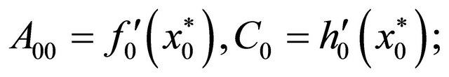
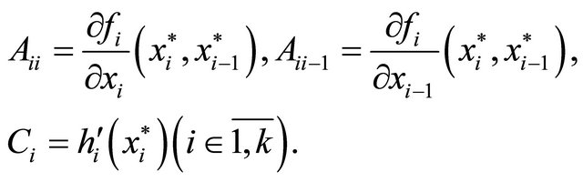
Define matrices  as follows:
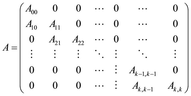 ,
,
 obtaining linear observation system
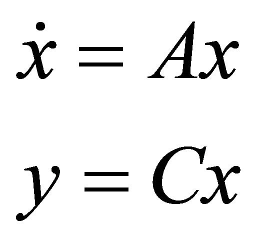 (LV)
(LV)
of verticum type (see [36]). In the latter paper, a Kalman-type necessary and sufficient condition for observability of linear verticum-type systems was obtained. Here we recall only its “sufficient part” to be applied below.
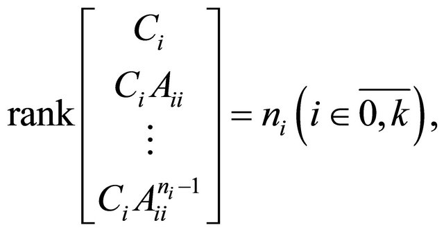
Theorem A.2. ([36]) Suppose that
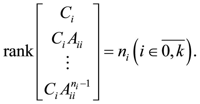
Then the linear verticum-type system (LV) is observable.
Remark A.5. If  is a Lyapunov stable equilibrium of system

then  can be considered as a control-observation system with “small” controls in the following sense. By the Lyapunov stability of
 , for all
  , there exists
  such that
  implies
 (for
(for ). In particular,
 for all
 .
.
Considering  as a control for system
  (Vi) becomes a controlobservation system in the sense of this Appendix. Suppose that for each
 then by Theorem A.2 the verticum-type system (LV) is observable.
Hence, the linearization of the observation system (V) is observable. Therefore, by Kalman’s theorem on observability of linear systems (see [1]), the rank condition  is fulfilled, which by Theorem A.1 implies local observability of system (V) near equilibrium
 .
.
The above reasoning can be summarized in the following theorem:
Theorem A.3. If equilibrium  is Lyapunov stable for system
  , and
, and
then observation system (V) is observable near its equilibrium .
.
NOTES
*Corresponding author.