American Journal of Operations Research
Vol. 2 No. 2 (2012) , Article ID: 19946 , 10 pages DOI:10.4236/ajor.2012.22026
An EPQ Model with Imperfect Production Systems with Rework of Regular Production and Sales Return
1Bharathiar University, Coimbatore, India
2Chickanna Government Arts College, Tirupur, India
Email: srivigneswar_ooty@yahoo.co.in
Received February 14, 2012; revised March 16, 2012; accepted March 31, 2012
Keywords: EPQ; Cost of Quality; Defective Items; Cycle Time; Rework; Sales Return; Demand and Production
ABSTRACT
The Economic Production Quantity (EPQ) model is commonly used by practitioners in the fields of production and inventory management to assist them in making decision on production lot size. The common assumptions in this model are that all units produced are perfect and shortages are not allowed. But, in real situation the defective items will be produced in each cycle of production and shortages and scrap are possible. These assumptions will underestimate the actual required quantity. Hence, the defective items can not be ignored in the production process. Rework process is necessary to convert those defective into finished goods. This study proposes EPQ model that incorporates both imperfect production quality and falsely not screening out a proportion of defects, thereby passing them on to customers, resulting in defect sales returns. To active this objective a suitable mathematical model is developed and the optimal production lot size which minimizes the total cost is derived. An illustrative example is provided and numerically verified. The validation of result in this model was coded in Microsoft Visual Basic 6.0.
1. Introduction
The primary operation strategies and goals of most manufacturing firms are to seek a high satisfaction to customer’s demands and to become a low-cost producer. To achieve these goals, the company must be able to effectively utilize resources and minimize costs. The Economic Production Quantity (EPQ) model is commonly used by practitioners in the fields of production and inventory management to assist them in making decision on production lot size. Classic EPQ model assumes that all items produced are of perfect quality and a continuous inventory issuing policy for satisfying product demand. However, in a real life production environment, due to controllable and/or uncontrollable factors, generation of defective items is inevitable and the defective rate cannot be ignored in the production process. Defective items will be produced in each cycle of production in most practical situations. It is clear that there are many instances in which the produced imperfect quality items should be reworked or repaired with additional costs. A portion of defective items produced are not successfully screened out internally during the production process and passed on to customers, thereby causing defect sales returns and reverse logistics from customers back to the manufacturer. Little research has addressed the important issues of handling sales return and/or various options of disposing of defects. A considerable amount of research has been carried out to address the problems of imperfect quality EPQ models. Several scholars have investigated the effect of imperfect quality production on economic production models. Gupta and Chakraborty [1] considered the reworking option of rejected items. They considered recycling from the last stage to the first stage and obtained an economic batch quantity model. Rosenblatt and Lee [2] assumed that the time from the beginning of the production run until the process goes out of control is exponential and that defective items can be reworked instantaneously at a cost and kept in stock. DaeSoo Kim et al. [3] presented a profit maximizing EPQ model that incorporates both imperfect production quality and two-way imperfect inspection, i.e. Type I inspection error of falsely screening out a proportion of non-defects and disposing of them like defects and Type II inspection error of falsely not screening out a proportion of defects, thereby passing on to customers resulting in defect sales returns. Maity et al. [4] presented an optimal control recovery production inventory system with shortages under inflation and discounting in fuzzy stochastic environment. The product defectiveness is random. The defective product also is treated as return product. Remanufactured product can be used for assembly of new products which is sold again and demand depends on the stock of serviceable product and time. Nita H. Shah et al. [5] developed an inventory model that jointly optimizes cost of manufacturer and retailer under buoyant market condition. Proposed model also considers imperfect production processes and partly backlogging is allowed only at the retailer’s end. Gour Chandra Mahata et al. (2010) developed an [6] developed an EPQ model for deteriorating items in the fuzzy sense where delay in payments for both retailer and customer are permissible to reflect realistic situations. Swapan Kumar Manna [7] developed two deterministic economic production quantity (EPQ) models for Weibull-distribution deteriorating items with demand rate as ramp type function of time. It is assumed that the finite production rate is proportional to the timedependent demand rate and the unit production cost is inversely proportional to the production rate. The EPQ model without shortages is studied first and with shortages is investigated next. Biswajit Sarkar et al. [8] developed an economic production quantity model for both continuous and discrete random demand of merchandise and a certain percent of the total product is of imperfect quality, which follows a probability distribution. The imperfect quality items are reworked at a cost. The percent of defectiveness in the total product usually increases with an increase in production run time. K. Srinivasa Rao et al. [9] concerned with a production inventory system with the assumption that the life time of the product is random and follows a Weibull distribution. This paper uses mathematical modeling to derive the long run average cost function for the proposed EPQ model with scrap, rework and sales return then employs optimality conditions to determine the optimal production quantity for the proposed mode. The remainder of the paper is organized as follows. Section 2 presents the assumptions and notations. Section 3 is for problem formulation and numerical example. Section 4 summarizes the assumptions. Finally, the acknowledgement of the author.
2. Assumptions and Notations
The following assumptions and notations are made to develop the model:
Assumptions: 1) A single type of product in a single stage production system is considered, 2) Production rate is constant and greater than demand rate, 3) Proportion of defective is constant and only one type of defective is produced in each cycle, 4) Defective items produced at the production process are reworkable and reworked items are either good items or scraps, 5) All demands must be satisfied, 6) Backlogging permitted, 7) Proportion of scrap is less than the proportion of defectives, 8) Inspection cost is ignored since it is negligible with respect to other costs, 9) Setup time for rework process is zero and 10) The other assumption in classical EPQ model.
Notations: P—Production rate in units per unit time, D—Demand rate in units per unit time, d—rate of defective items from regular production (d = Px), w—rate of defective items from end customers in units (w = Dy), —on hand inventory level, Q*—Optimal size of production run,
 —Setup cost,
 —Holding cost per unit/year,
 —Cost of quality improvement,
 — Cost of reworking per unit,
 —Cost of rejecting per unit,
 —Production Cost per unit,
 —Proportion of defective items that cannot be reworked (scrap item), x—Proportion of defective items from regular production (X is between 0 to 0. 1), y—proportion of defective items from customers (y is between 0 to 0.1) and T—Cycle time and
 —unit time periods i (i = 1, 2, 3, ···).
3. Mathematical Model
A real-life production process due to process deterioration or other factors may generate randomly x per cent of defective items at a production rate d. Not all of the defective items produced are reworked. A portion  of the imperfect quality items are scrap and must be discarded before the rework process starts. The other (1 –
 ) portion of imperfect items is reworked at a rate of P immediately after the regular process. Stockout situation is allowed. Shortages are backordered and satisfied by the immediate next replenishment. In this case, scrap can be detected before the rework process starts to produce good items from the defectives. Figure 1, shows inventory when defective items are reworked within the cycle and are detected before rework starts.
  are the time segments, which represents the processing time (uptime), rework time without scrap and down time (or) consumption time respectively. From the beginning to the end of the production process both good and defective items are
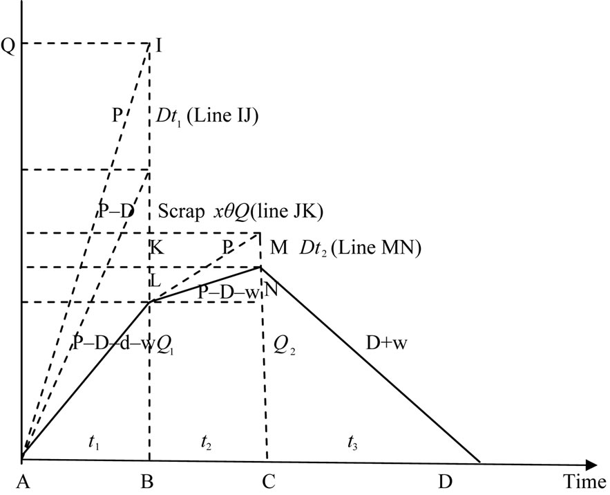
Figure 1. On-hand inventory of perfect quality items in EPQ model with Scrap and rework.
produced at a rate of x during time . The line AO indicates the slope of
  and inventory is increasing at the rate of P, simultaneously decreasing at the rate of D + d as demand and w as a sales return from the customers. Then the inventory accumulates at the rate of
 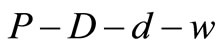 units. Therefore, the net amount of defectives produced during time
  is xQ. It is assumed that
  percent of defectives is scrap. Hence, at the end of time
 , the scrap units
  are identified and separated from the main inventory say line JK indicates that amount. The remaining defective Qx(1 –
 ) units are reworked at the rate of P units/year, as the rework rate is assumed as the same as production rate. On hand inventory of defective items during production uptime
  and reworking time
  shows that maximum level of onhand defective items is dt1 and
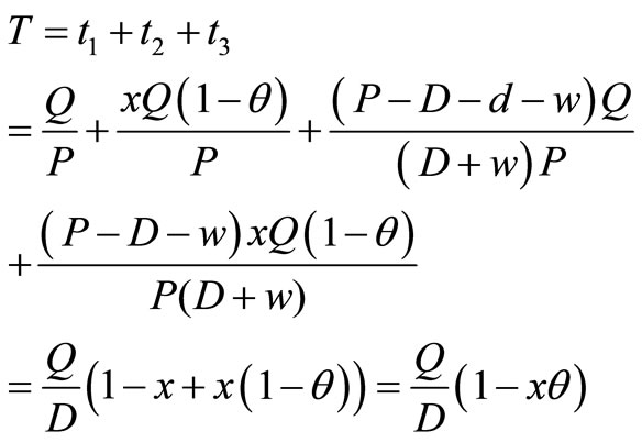
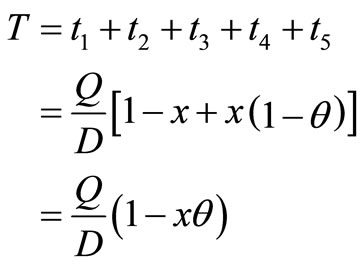
 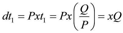 . According to the definition, DT = Q, therefore
  and Q = Pt1, therefore,
  .
.  represents the quantity of good items remaining after consumption at the end of time
 ,
,  represents the quantity of items that should remain after consumption if no defective items is produced at the end of time t1. From the Figure 1 hence, it can be shown that
Time  needed to rework the defective items
Time t3 needed to built up Q2 units of items, therefore,
Inventory during production cycle time
Note: When , then
  which is the standard inventory model.
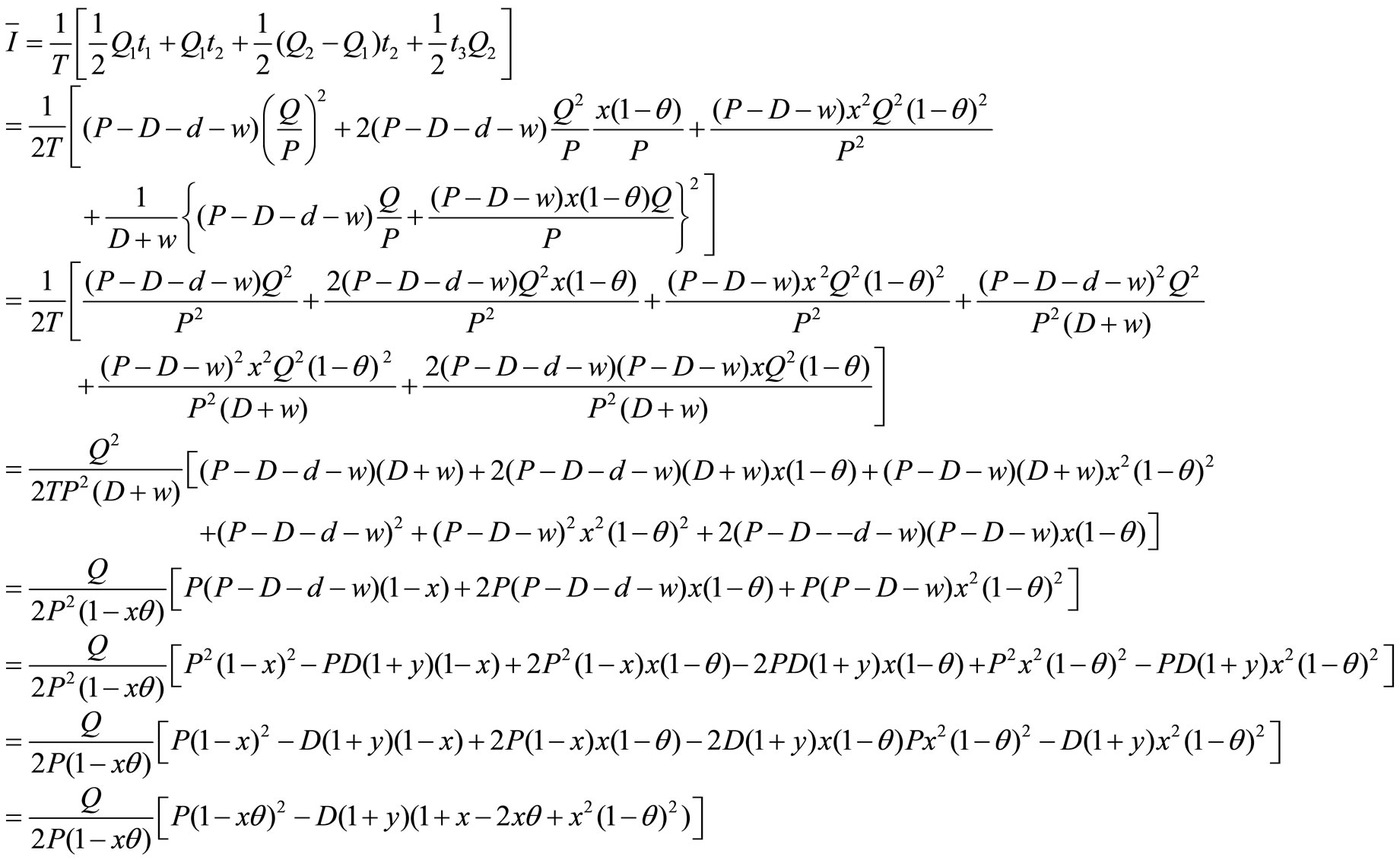
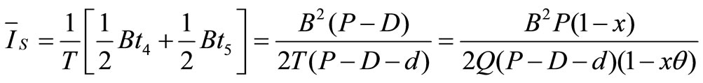
Average Inventory Calculation: The average inventory is calculated as follows from the Equations (1) to (6):
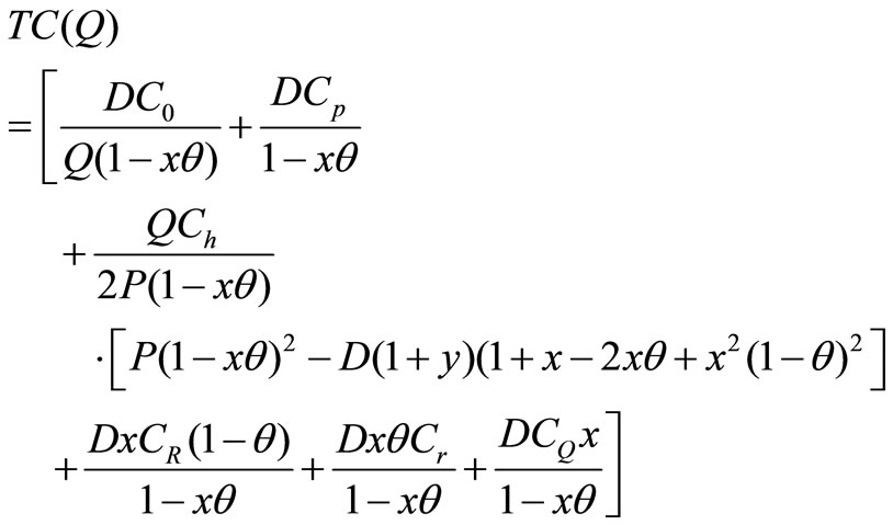
Total Cost: Generally the total cost of a production system consists of three major costs. Such as setup cost, Process Cost, Inventory Carrying cost. The total cost of the system TC(Q), is the accumulation of the setup cost, production cost, inventory holding cost, reworking due to reworking. But in this research, the total cost of the system TC(Q) is the accumulation of the Setup Cost, Production cost, holding cost, Reworking cost, Rejecting cost and Quality cost for defective items.
1. Setup cost = 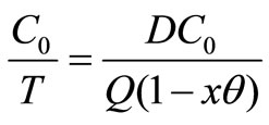
2. Production cost per unit time = 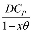
3. Inventory carrying cost = 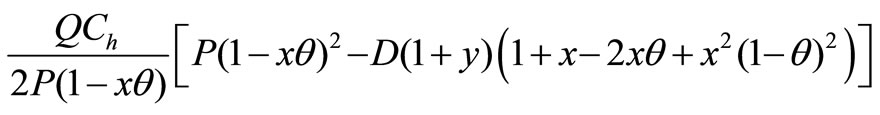
4. Reworking cost/time = 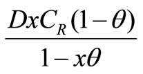
5. Rejection cost per unit time = 
6. Quality cost = 
Therefore,
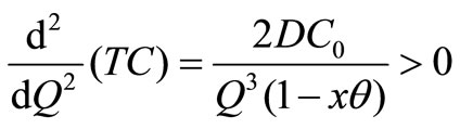
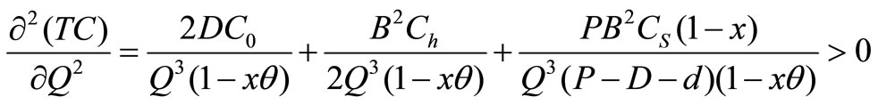
Optimality: It can be easily shown that TC(Q) is a convex function in Q. Hence, an optimal production quantity Q*, can be calculated from 
which yields
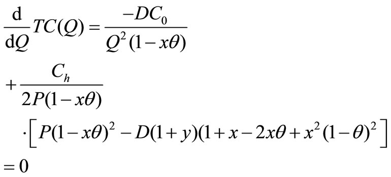
Therefore Q* =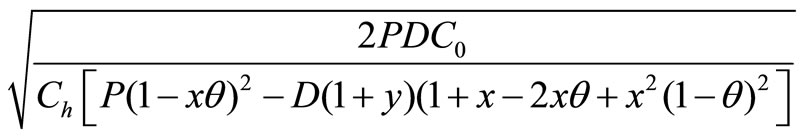
Numerical Example: The solution above is validated through numerical examples in the following section.
Let P = 5000 units; D = 4500 units;  = 100;
 ;
; ;
;
 ;
;  x = 0.01 to 0.09, y = 0.01 to 0.1 and
 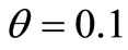 to 0.9.
Optimum Solution: Q = 1049.84;  = 85.04; Q2 = 85.90; Setup Cost = 429.06; Production cost = 450, 450.45;
Holding cost = 429.06; Reworking cost = 202.70; Rejecting = 4.50; Quality Cost = 225.22, Total cost = 451741.00 Cycle Time Verification: To verify the model, t1 + t2 + t3 = 0.2100 + 0.0019 + 0.0212 = 0.2331 years. From equation of cycle time, it is also found that T = 0.2331 years which proves the model.
From the Table 1, it is observed that when the rate of defective (x) during production increases, then the optimum quantity (Q*), cycle time (T), production cost, Reworking cost, cost of rejecting, quality cost and total cost increases but setup cost and holding cost decreases. Therefore, there is direct relationship between rate of defective with optimum quantity, cycle time, production cost, reworking cost, cost of rejection, quality cost and total cost. But, there is inverse relationship between rate of defective items and setup and holding cost.
From the Table 2, it is observed that when the rate of sales return (y) increases, then the optimum quantity (Q*), cycle time (T), production cost, Reworking cost, cost of rejecting, quality cost and total cost increases but setup cost and holding cost decreases. Therefore, there is direct relationship between rate of defective with optimum quantity, cycle time, production cost, reworking cost, cost of rejection, quality cost and total cost. But, there is inverse relationship between rate of defective items and setup and holding cost.
4. Sensitivity Analysis
The total cost functions are the real solution in which the model parameters are assumed to be static values. It is reasonable to study the sensitivity i.e. the effect of making chances in the model parameters over a given optimum solution. It is important to find the effects on different system performance measures, such as cost function, inventory system, etc. For this purpose, sensitivity analysis of various system parameters for the models of this research are required to observe whether the current solutions remain unchanged, the current solutions become infeasible, etc.
Observations: From the Table 3, it has been observed that
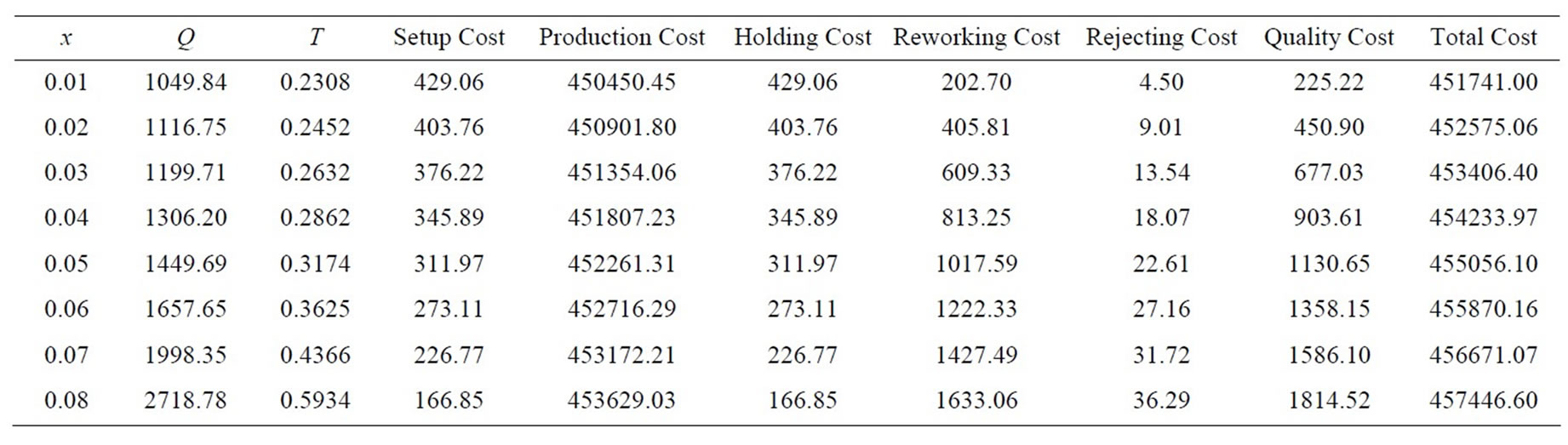
Table 1. Variation of rate of defective during production and optimum values.
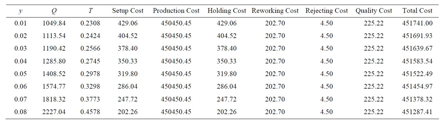
Table 2. Variation of rate of sales return and optimum values.
Table 3. Effect of inventory parameters with optimal values.
1) Increase in rate of production defective items (x), optimum quantity (Q*), production time (t1), cycle time (T) and total cost also increases but maximum inventory  decreases. 2) Increase in rate of sales return (y), optimum quantity (Q*), production time (t1), cycle time (T) and total cost also increases but maximum inventory
  decreases. 3) Increase in setup cost per unit (C0), optimum quantity (Q*), maximum inventory
  and
and , Production time (t1), cycle time (T) and total cost also increases. 4) Increase in holding cost per unit (
 ), optimum quantity (Q*), maximum inventory
  and
and , production time (t1) and cycle time (T) decreases but total cast also increases. 5) Similarly, other parameters a, production cost, reworking cost, rejecting cost, and quality cost can also be observed from the Table 2.
Special Cases:
Case (i): If the production system is considered to be ideal that is no defective items are scrap are produced, means the value of x, y and  is set to zero. In this case, the above equation reduces to the classical economic batch quantity model as follows: Therefore, Q* =
 .
.
Consider the above numerical example, therefore, the optimum solution is
Optimum Solution for Case (i):
Q = 948.68;  = 94.87;
  94.87;
 = 0.1897;
  = 0;
= 0;  0.0211; t = 0.2108 cycle time verified. Setup cost = 474.34; Production cost = 450,000; Holding cost = 474.34; Total cost = 450948.68.
Case (ii): When the defective items are produced and scrap is not and y = 0, the equation reduces to the economic batch quantity model with defective as follows:
Therefore, Q* = 
Consider the above numerical example, therefore, the optimum solution is
Optimum Solution for Case (ii):
Q = 994.98; ;
; ;
;
Setup cost = 452.27; Production cost = 450,000; Holding cost = 452.27; Reworking cost = 225; Rejecting cost = 0; Quality cost = 225; Total cost = 451354.54.
5. An EPQ Model with Imperfect Production Items, Rework of Regular Production with Shortages and Sales Return
Figure 2, depicts the on-hand inventory level and allowable backorder level for the EPQ model with backlogging permitted. One can obtain the cycle time T, production uptime , on-hand inventory level
  and
and , time needed to rework defective items
 , production downtime
 , Shortage permitted time
  and
and  as follows: According to definition: DT = Q, therefore, T =
 and Q =
 , therefore,
 .
.
 represents the quantity of good items remaining after consumption at the end of time
 .
.
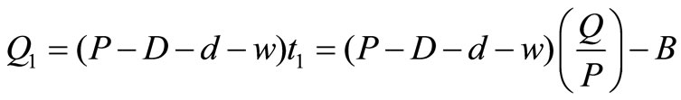
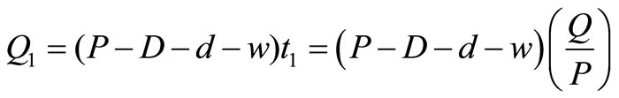
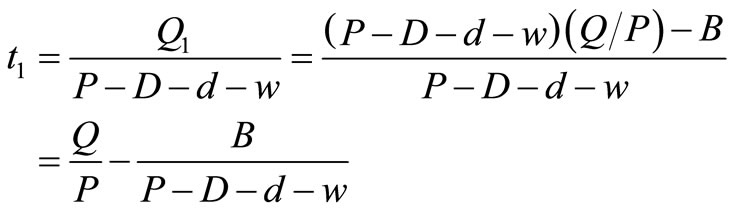
Time t1 needed to built up Q1 units of item, therefore,
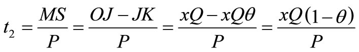
Time  needed to rework the defective items
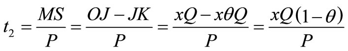
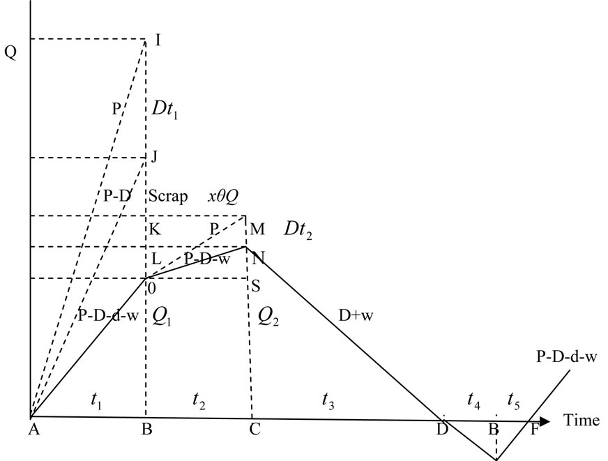
Figure 2. On-hand inventory of EPQ model with the rework and shortages permitted.
 represents the quantity of items that should remain after consumption
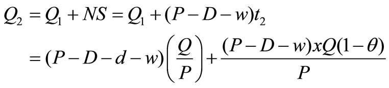
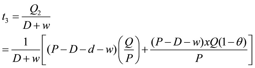
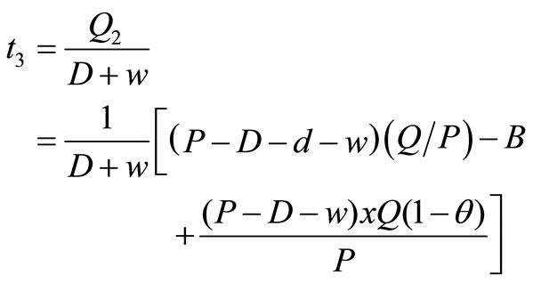
Time  needed to built up
  units of items, therefore,
Shortages time,  and
and 
Inventory during production cycle time,
Note: When x =  then
then  which is the standard inventory models.
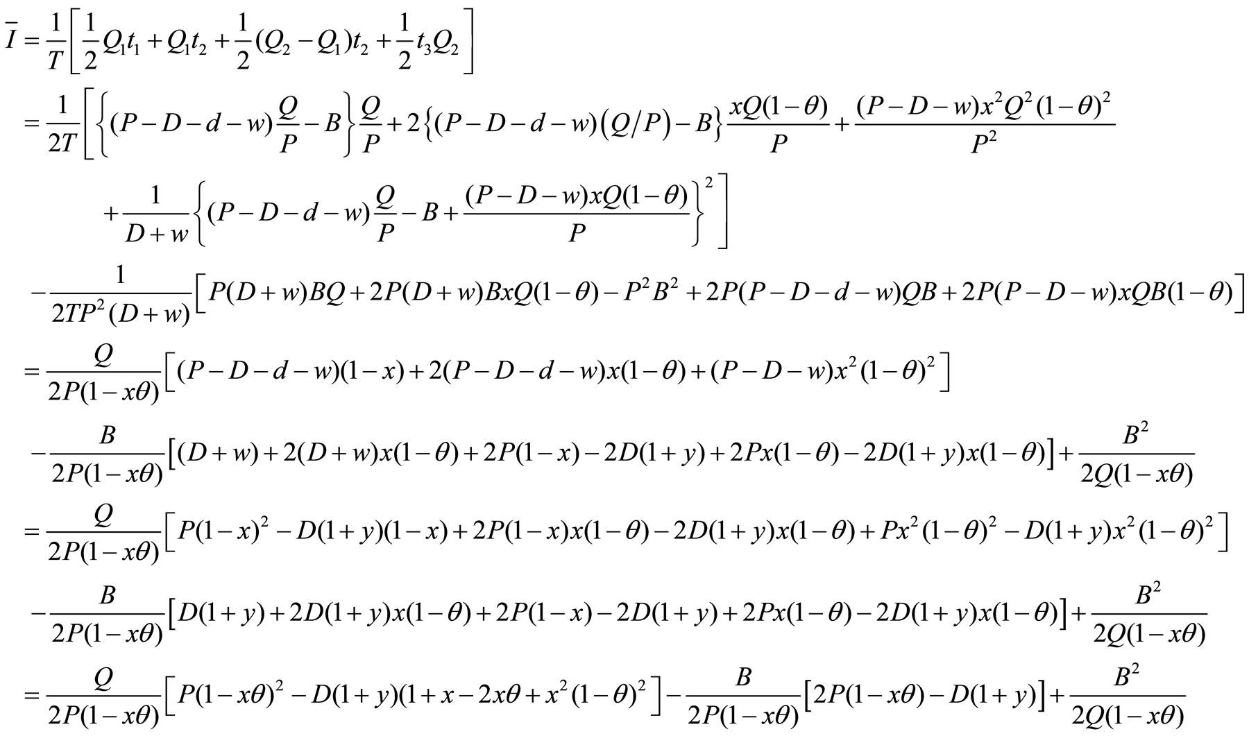
The average inventory is calculated as follows
Note: When x = y = = 0, then
 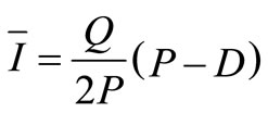 which is the standard inventory model.
The average inventory during shortage period is as follows:
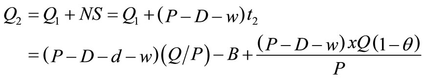
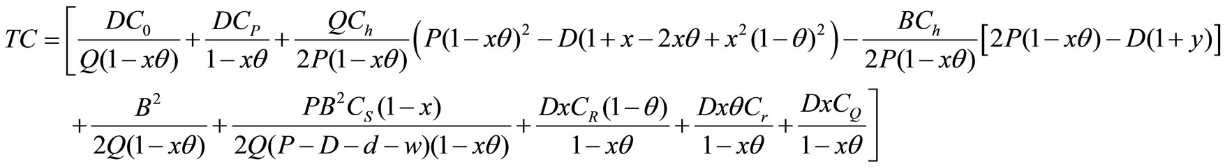
Total Cost (Q,B): The total cost of the system TC (Q,B) is the accumulation of the setup cost, production cost, holding cost, shortage cost, reworking cost, rejection cost and quality cost for defective items. Therefore, the total cost TC (Q,B) is
Partially derivative TC (Q,B) with respect to Q and B,

Let 
Therefore, 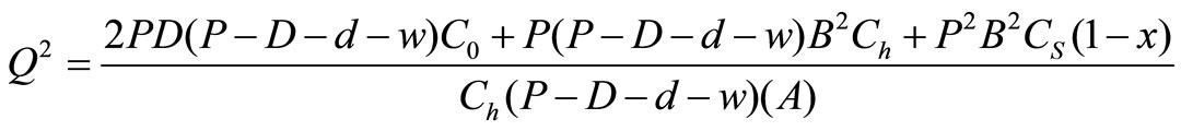

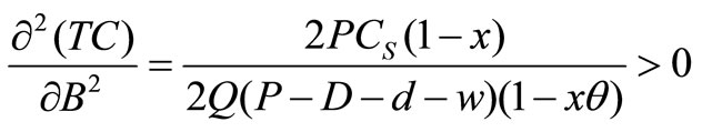
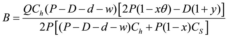
Therefore, the optimum lot size is
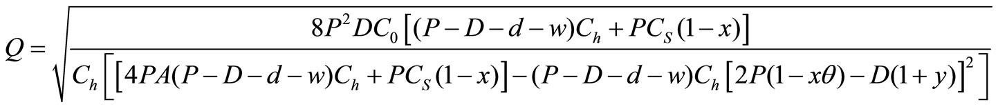
Numerical Example
Let the inventory system has the following parameter values Let P = 5000 units; D = 4500 units;  = 100;
  ;
; ;
;
 ;
; .
.
x = 0.01 to 0.09, y = 0.01 to 0.10 and  0.1 to 0.9;
 .
.
Optimum Solution
Q = 1232.65; B =50.76;  49.08;
  50.09;
Setup cost = 365.45; Production cost = 450450.45, Holding cost = 237.56;
Reworking cost = 202.70, Rejecting cost = 4.50; Quality cost = 225.22Shortage cost = 127.87, Total cost = 451613.75.
Cycle Time Verification:
To verify the model, it is calculated that
 0.1225;
  0.0023;
  0.0110,
  0.0111,
  = 0.1241 and T = 0.2710.
Therefore,  = 0.1225 + 0.0023 + 0.0110 + 0.0111 + 0.1241 = 0.2710which is equal to value of T. It proves the model.
From the Table 4, it is observed that when the rate of defective (x) during production increases, then the optimum quantity (Q*), cycle time (T), production cost, Reworking cost, cost of rejecting, quality cost and total cost increases but shortage cost, setup cost and holding cost decreases. Therefore, there is direct relationship between rate of defective with optimum quantity, cycle time, production cost, reworking cost, cost of rejection, quality cost and total cost. But, there is inverse relationship between rate of defective items with shortage cost, setup and holding cost.
6. Conclusion
In practices, production and screening processes of a
Table 4. Variation of rate of defective items from regular production with inventory and total cost.
manufacturer are not perfect, thereby producing and passing some defects to customers. Most of the existing imperfect quality inventory models, however, have not dealt with such important practical situations involving both imperfect production and imperfect screening process. The falsely screening out a proportion of defects, thereby passing them on to customers and consequently resulting in customers defect sales returns due to quality dissatisfaction. Therefore, this paper present a imperfectquality inventory model and defect sales return that determines an optimal production lot size. Some numerical examples were carried out to illustrate the models. Result validation is a necessary step in this research. For validation, the model was coded in Microsoft Visual Basic 6.0. The proposed model can assist the manufacturer and retailer in accurately determining the optimal quantity, cycle time and inventory total cost. Moreover, the proposed inventory model can be used in inventory control of certain items such as food items, fashionable commodities, stationary stores and others.
7. Acknowledgements
The author greatly appreciates the editor and the anonymous referees for their valuable comments and suggestions to improve the paper in the present form. This research work is fully related to my Ph.D. work in Mathematics and which is to be submitted to Bharathiar University.
REFERENCES
- T. Gupta and S. Chakraborty, “Looping in a Multistage Production System,” International Journal of Production Research, Vol. 22, No. 2, 1984, pp. 299-311. doi:10.1080/00207548408942455
- M. J. Rosenblatt and H. L. Lee, “Economic Production Cycles with Imperfect Production Processes,” IIE Transactions, Vol. 8, No. 1, 1986, pp. 48-55.
- S. H. Yoo, D. Kim and M. S. Park, “Economic Production Quantity Model with Imperfect Quality Items, Two Way Imperfect Inspection and Sales Return,” International Journal of Production Economics, Vol. 121, 2009, pp. 255-265.
- A. K. Maity, K. Maity and M. Maity, “Optimal Remanufacturing Control Policy with Defective Item,” International Journal of Operation Research, Vol. 6, No. 4, 2009, pp. 500-518. doi:10.1504/IJOR.2009.027155
- N. H. Shah, A. S. Gor and C. Jhaveri, “Joint Optimal Production Inventory Model with Imperfect Production Processes and Varying Deterioration Rate in Buoyant Market,” International Journal of Operational Research, Vol. 9, No. 2, 2010, pp. 125-140. doi:10.1504/IJOR.2010.035041
- C. Mahata, et al., “The Optimal Cycle Time for EPQ Inventory Model of Deteriorating Items under Trade Credit Financing in the Fuzzy Sense,” International Journal of Operations Research, Vol. 7, No. 1, 2010, pp. 26-40.
- S. K. Manna and C. Chiang, “Economic Production Quantity Models for Deteriorating Items with Ramp Type Demand,” International Journal of Operational Research, Vol. 7, No. 4, 2010, pp. 429-444. doi:10.1504/IJOR.2010.032420
- B. Sarkar, S. S. Sana and K. Chaudhuri, “An Economic Production Quantity Model with Stochastic Demand in an Imperfect Production System,” International Journal of Services and Operations Management, Vol. 9, No. 3, 2011, pp. 259-283. doi:10.1504/IJSOM.2011.041100
- K. Srinivasa Rao, S. V. Uma Maheswara Rao and K. Venkata Subbaiah, “Production Inventory Models for Deteriorating Items with Production Quantity Dependent Demand and Weibull Decay,” International Journal of Operational Research, Vol. 11, No. 1, 2011, pp. 31-53. doi:10.1504/IJOR.2011.040327