Journal of Electromagnetic Analysis and Applications
Vol.09 No.10(2017), Article ID:80046,12 pages
10.4236/jemaa.2017.910012
Point Charges and Conducting Planes for Yukawa’s Potential and Coulomb’s Potential
M. A. López-Mariño1*, Juan C. Trujillo Caballero2
1Tecnológico de Monterrey, Escuela de Ingeniería y Ciencias, Chihuahua, Chihuahua, México
2Instituto Tecnológico de Orizaba, Departamento de Ingeniería Eléctrica, Orizaba, Veracruz, México

Copyright © 2017 by authors and Scientific Research Publishing Inc.
This work is licensed under the Creative Commons Attribution International License (CC BY 4.0).
http://creativecommons.org/licenses/by/4.0/


Received: July 28, 2017; Accepted: October 28, 2017; Published: October 31, 2017
ABSTRACT
In this work, we modeled and simulated the electric potential generated by point charges in the region of grounded conductor planes for Yukawa potential and Coulomb potential . We show the symbolic expression for the electric potential and some graphs for it and for the electric field with different values of . We observe that the electric potential decreases as the value of increases and that does not allow all the charge to be distributed on the surface of the conductor.
Keywords:
Yukawa Potential, Coulomb Potential, Method of Images

1. Introduction
In every electromagnetic theory course, from elementary to advanced ones, electrostatic problems are analyzed. Such problems require finding the functions describing potential and electric field in the region close to the charge distributions, bound to the boundary conditions imposed by the problem’s geometry. This kind of problems are usually modelled using Poisson’s equation
(1)
Most exercises involving practical applications require students to know how to solve differential equations in partial derivatives. However, while taking elementary electricity and magnetism courses, students lack this knowledge or any alternative one such as numerical analysis. A simple procedure, capable of overcoming the aforementioned obstacle, is provided by the Method of Images (MI), which is normally used in problems featuring spatial symmetry. Nevertheless, its use for the most difficult cases can turn out to be so complicated that it loses practicality. Under this method [1] [2] [3] [4] , the first step is to determine the
electrical potential from , in the case of Coulomb’s potential used in
electromagnetic courses. Then, the electric field can be obtained in the usual way .
According to the MI, a configuration featuring a charge close to an infinite conductive plane, correctly grounded can be replaced by the charge configuration, its image and an equipotential surface substituting the conductive plane.
When charges are present, in order to comply with both Poisson’s equation and boundary conditions, the method requires:
1) The charges and their images to be located in the conductive plane region;
2) The charges and their images to be arranged in such a way that, within the conductive plane, the potential be zero or constant.
The procedure is a very valuable aid since it does not require advanced math knowledge nor complex algorithms; all it requires is a knowledge of the expression for some basic electric potentials as well as the one for the superposition principle.
In an interesting work, Griffiths and Uvanovic [5] studied the charge distribution on a conductor for two potentials: Yukawa potential and the Law of Potential .
Unlike Coulomb potential, where the entire charge is distributed on the surface, they found that under Yukawa’s a portion of the charge goes to the surface while the rest is evenly distributed in its volume. As for the Law of Potential, they did not reach a general result. Later on, Sallabi et al. [6] used MI to study charge distribution in conductors using Yukawa potential. For the Yukawa potential, Equation (1) is generalized to [5]
(2)
The aim of this work is to apply MI to a typical problems dealing with point charges and grounded conductive planes in order to find the total potential and electric field, using as interaction among charged particles Yukawa and Coulomb potentials. When obtained through this method, potentials can be established in terms of elemental functions. Its analytical expressions and graphs can be shown using Maple. The expressions of the electric field can be long and therefore we do not include them in this work. Nevertheless, the reader can use Maple’s instructions in Appendix A and Appendix B to calculate the expressions for the potential and the electric field as well as the graphs shown.
The current work is composed as follows: In Section 2, we discuss the case of a point charge located in the region over a grounded plane conductor; In Section 3, we present the case of two grounded conducting planes, perpendicular to each other and a point charge placed in a quadrant between the planes; In Section 4, our final comments are presented.
2. Point Charge and a Conducting Plane
In this section, we determine the potential produced by a positive charge Q, located at a distance d on a very large and grounded conducting plane, as shown in Figure 1.
To find the potential in the region and to guarantee that the potential in the plane is zero, it is necessary to replace the conducting plane by an image charge −Q, located in , as shown in Figure 2. A point is defined, on which we aim to calculate the potential.
From the problem’s geometry, it is established that
(3)
Hence, the potential produced on P, due to Q, is given by
(4)
Similarly, we are able to find, for the image charge,
(5)

Figure 1. Grounded plane and point charge.

Figure 2. Q charge and its image.
which means the potential it produces on P is given by
(6)
Following the superposition principle, it is possible to express the resulting potential on point P as the sum of and ; that is to say,
(7)
The expression for potential obtained using Maple are given [7] [8] by
(8)
which matches (7) when .
For the following graphics, we set the values for the distance between the plane and the charge as and the charge was given a value of . Then we used the Maple to generate the plots [7] [8] (See Appendix A).
Figure 3(a), shows the Coulomb’s potential produced by the charge; it can be seen that it meets the boundary condition, . Figure 3(b) shows additionally the field lines that perpendicularly intersect the equipotential curves.
In the case of Yukawa, the expression for potential obtained with Maple is

Figure 3. (a) Coulomb potential, and (b) Potential and electric field.
(9)
Figure 4 shows Yukawa potential for ; some field lines are also shown.
It is observed that the potential decreased and, therefore, the boundary condition in the conducting plane is not satisfied.
3. Point Charge between Two Perpendicular Conducting Planes
In this section we calculate the potential and electric field produced by a point charge Q, placed at the point whose coordinates are between two grounded perpendicular conducting planes as shown in Figure 5.

Figure 4. (a) Yukawa’s potential for , and (b) Potential and electric field.

Figure 5. Q charge between two perpendicular planes.
Similarly to the single plane case, in order to ensure that the potential is zero at the horizontal plane, it is necessary to place a image charge −Q under the plane, at . However, since this does not guarantee that the potential above the vertical plane is zero, we add a image charge −Q to the left of such plane, at ; this makes the potential at the horizontal plane different from zero. Finally, to comply with the boundary condition of zero potential in both planes, we place a Q charge in . The point charge Q and its image charges are shown in Figure 6.
By the superposition principle, we find the resulting potential on point P as
(10)
With the expression for potential that we got using
Maple is given [7] [8] by
(11)
To graphically illustrate the total Coulomb potential, the equipotential curves and the electric field were plotted using Maple in the region where y , we considered the values for the position of the charge (1,1,0) as well as its magnitude and we used Maple [7] [8] (See Appendix B).

Figure 6. Q charge and its image charges.
Figure 7(a) shows the resulting potential; we can see finite values except for the potential at the point , which is where the charge is placed. It is observed that the potential satisfies the boundary condition with each of the planes. Figure 7(b) shows the electric field in addition to the potential.
In the case of Yukawa, the potential is given by
(12)
Figure 8 shows Yukawa potential for ; some field lines are also shown.
In this case, it is also observed how the potential decreased and no longer satisfies the boundary conditions.
4. Concluding Remarks
Two simple and well-known arrays of charges and conducting planes have been analyzed through the MI [7] [8] . The number of necessary image charges, N, to satisfy boundary conditions depends on the separation angle between the semiinfinite planes and can be calculated with the following relation [2]
(13)
where . In the case presented in Figure 1, and image

Figure 7. (a) Coulomb’s potential, and (b) Potential and electric field.

Figure 8. (a) Yukawa’s Potential for μ = 5, and (b) Potential and electric field.
charge is necessary; when as in Figure 5, image charges are necessary.
For this work, we used the MI and Yukawa’s potential as a generalization of the electrical potential produced by a point charge in the vicinity of grounded conducting planes; as a particular case, we obtained its Coulomb’s potential. Yukawa potential decreases exponentially depending on the value of μ and, therefore, and so does the resulting electric field, which was expected. This explains why, in solid conductors, the charge does not fully flow to the surface [5] [6] and why, in the Coulomb limit ( ), we get the well-known result where the entire charge reaches the surface.
We are interested in our students experiencing not only the simulation of potentials and electric fields, but also their modeling. We think that both elements, modeling and simulation [9] [10] , can motivate them to reach numerical results, as well as to suggest simple analytical and computational procedures. Such combination should contribute to their getting an integral learning experience. Although both quantities, potential and electric field, could be expressed in terms of elementary functions, the support of a computational tool was very stimulating, particularly for engineering students, who fully appreciate, in addition to numerical values, the graphs that foster the learning of concepts. Finally, we, as professors in charge of elementary courses, are able to address more interesting and difficult problems than those usually solved during electricity and magnetism courses without the hindrance of demanding advanced mathematics or programming knowledge from the students.
Acknowledgements
We would like to express our gratitude to Professors N. Aquino from Universidad Autónoma Metropolitana, Iztapalapa, G. Maldonado from Tecnológico de Monterrey, Campus Central de Veracruz and L. M. Orona from Tecnológico de Monterrey, Campus Chihuahua, for careful reading of the manuscript and for valuable comments on this work.
Cite this paper
López-Mariño, M.A. and Trujillo Caballero, J.C. (2017) Point Charges and Conducting Planes for Yukawa’s Potential and Coulomb’s Potential. Journal of Electromagnetic Analysis and Applications, 9, 135-146. https://doi.org/10.4236/jemaa.2017.910012
References
- 1. Cheng, D.K. (1992) Field and Wave Electromagnetics. 2nd Edition, Addison-Wesley Publishing Company, New York.
- 2. Sadiku, M.N.O. (2002) Elements of Electromagnetism. 3rd Edition, Oxford University Press, Inc., New York.
- 3. Clayton, R.P. and Nasar, S.A. (1987) Electromagnetic Fields. 2nd Edition, McGraw-Hill, New York.
- 4. Shen, L.C. and Kong, J.A. (1987) Applied Electromagnetism. PWS Publishers, Boston.
- 5. Griffiths, D.J. and Uvanovic, D.Z. (2001) The Charge Distribution on a Conductor for Non-Coulombic Potentials. American Journal of Physics, 69, 435. https://doi.org/10.1119/1.1339279
- 6. Sallabi, A.K., Khaliel, J.A. and Mohamed A.S. (2014) Method of Images to Study the Charge Distribution in Cases of Potentials Deviating from Coulomb’s Law. Journal of Electromagnetic Analysis and Applications, 6, 51-56. https://doi.org/10.4236/jemaa.2014.64008
- 7. Bueno Pascual, F.E., López-Mariño, M.A. and Aquino N. (2007) Potencial y campo eléctrico generados por una carga puntual entre dos planos conductores aterrizados In: L Congreso Nacional de Física, Veracruz, Veracruz , 227.
- 8. López-Mariño, M.A. and Aquino, N. (2015) Cálculo del potencial y del campo eléctrico producido por una carga puntual y planos conductores. In: LVIII Congreso Nacional de Física, Mérida, Yucatán, 270.
- 9. López, S., Veit, E.A. and Araujo, I.S. (2016) A Literature Review about Computational Modeling and Simulation in Physics Education in Middle and High School Levels. Revista Brasileira de Ensino de Física, 38, e2401.
- 10. López-Mariño, M.A., Hernández-Olvera, J.A., Barroso, L.A. and Trujillo Caballero, J.C. (2017) Graphic and Symbolic Computation: Analysis on the Spring-Mass System. Revista Brasileira de Ensino de Física, 39, e2303.
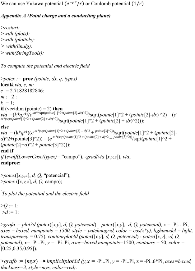
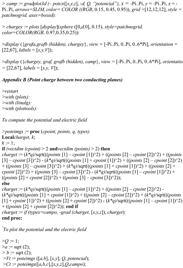
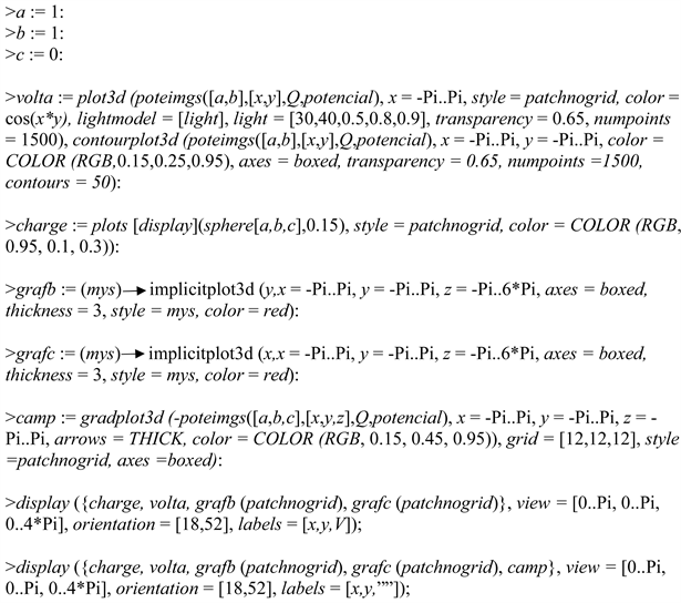
Appendices