Journal of Electromagnetic Analysis and Applications
Vol.4 No.3(2012), Article ID:18221,7 pages DOI:10.4236/jemaa.2012.43013
Wideband Modeling of Land-Mobile-Satellite Channel in Built-Up Environment
![]()
1Electrical and Computer Engineering Department of University of Nizwa, Nizwa, Sultanate of Oman; 2Electrical Engineering Department of Jordan University of Science and Technology, Irbid, Jordan; 3Computer Engineering Department of Hodeidah University, Hodeidah, Yemen.
Email: jarndal@ieee.org
Received January 17th, 2012; revised February 13th, 2012; accepted February 22nd, 2012
Keywords: Radio Channel Modeling; Electromagnetic Wave Propagation; Satellite Mobile Communication; Ray Tracing; Uniform Theory of Diffraction
ABSTRACT
This paper presents a propagation model for land-mobile-satellite (LMS) wideband radio channel in built-up environment. The model characterizes the behavior of the radio channel, under shadowing and multipath effects due to buildings, with variation of the elevation angle of the satellite. The wideband parameters (coherent bandwidth and time delay spreading) for LMS channel, in residential and urban environments, are computed. These parameters can be considered as a measure of the amount of ISI (inter-symbol interference) of the radio channel, which distorts the received signal and accordingly increases the bit error rate. The calculated values for these parameters using our model, show very good agreement with the corresponding measured ones, which accordingly shows the validity of the developed model for radio channel design in satellite mobile communication systems.
1. Introduction
Mobile satellite communication systems are designed to provide truly global coverage using constellation of low, medium, or geostationary earth orbit satellites. These systems may suffer from poorer quality of service due to high free-space path loss, tree or hills shadowing and multipath due to structures in the vicinity of the mobile. The first two effects mainly influence the line-of-sight LOS (or the direct) path and result in large scale fading, which causes severe signal attenuation especially at small satellite elevation angles. The last one is responsible for small scale fading and time spreading in the received signal, which occurs due to the vector addition of reflections, diffractions and scattering from local objects such as buildings [1]. Statistical approaches have been used for modeling the LMS channel [2]. These model are simpler, however, due to lack of physical background, such models may provide unreliable results. On the other hand, deterministic models provide high accuracy, but they require actual analytical path profiles and timeconsuming computations [3]. A combination of both approaches has been also developed [4]. In general these models can be classified in to narrowband and wideband models. The first one is concerned with voice/data applications of smaller signal bandwidth with respect to the coherent band-width of the channel [5,6]. Lower attention has been given for wideband modeling of LMS channel, which becomes critically required for multimedia applications of higher bit rate. Sine, time spreading in the order of 10 ns is a very important factor to be considered for application of bit rate ≥ 10 Mb/s. In these cases, deterministic ray-tracing based models, which describe the area around the mobile could be very efficient to estimate the amount of inter-symbol interference (ISI) and thus the associated bit error rate.
Wideband characterization of LMS channel has been presented in different papers. In [7] the received signal was measured for different elevation angles and environments. UTD (uniform theory of diffraction) based propagation model including only single edge diffraction was reported indeed [8]. The main contribution of this paper with respect to the last reported one in [5] is the improved modeling procedure with higher emphasis on the time delay of each ray contribution with respect to the minimum delay (direct) path. Thus the main features of the developed wideband model are:
1) Accurate description of multipath effects by including all expected contributions like building edge diffractions, building wall reflections, ground reflections, multiple reflections, multiple diffractions, and multiple reflections-diffractions.
2) Calculating the received signal at the mobile with variation of the elevation angle of the satellite.
3) Computing time-variant impulse response and transfer function of the satellite-to-mobile radio channel.
4) Deriving power delay profile (PDP) for the multipath LMS channel, in addition to the root-mean-square time delay (trms).
5) Providing simulation results that have a very good agreement with corresponding measured ones in [7] and [9].
2. System Propagation Model
The model is adopted to characterize only the multipath mechanism around the mobile, which is the main cause of the received signal fast fading and time spreading (distortion). Accordingly, the model will calculate the normalized amplitude of the received multipath signal at the mobile with respect to the received direct one above the building. The geometry of the propagation model is illustrated in Figure 1. A satellite moving in circular orbit above the surface of the earth descends behind a row of buildings of height hb and width wb. A mobile antenna located at a height hm above the ground is at a distance xm away from the building. The received signal at the mobile antenna is estimated for satellite elevation angles, 0˚ < q < 180˚. The carrier frequency of 2.5 GHz was assumed for the transmitted signal from the satellite to the mobile.
3. Wideband Characterization
Multipath wideband channel can be considered as a timevariant system. The effects of scatterers in discrete delay ranges are lumped together into individual “tap” with the same delay. Each tap represents a single ray contribution to the received signal and has gain, which varies in time
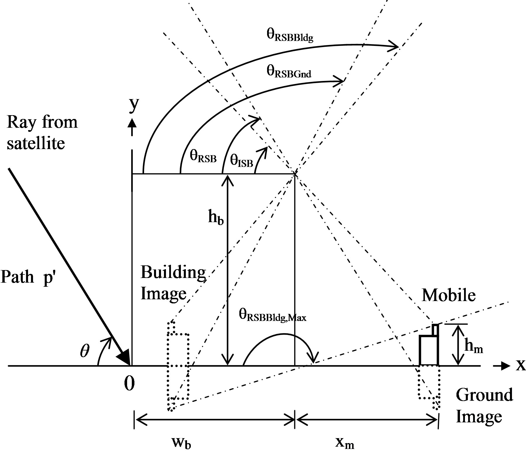
Figure 1. Zones for ray contributions due to building blockage.
according to the standard narrowband channel statistics [5]. The taps are usually assumed to be uncorrelated from each other. Since each tap arises from scatterers, which are physically distant and separated by many wavelengths. The basic function that characterizes the channel is the time-variant impulse response. The channel is therefore a linear filter with a time-variant finite impulse response as illustrated in Figure 2. The output Y(t) at a time t for input U(t) can be determined by convolving the input with the impulse response
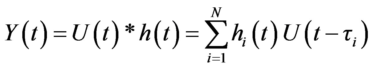 (1)
(1)
where * denotes convolution and τ is the delay variable.
3.1. Radio Channel Transfer Function and Impulse Response
The LMS radio channel can be considered as a time variant system because the characteristic of the channel changes with variation of the elevation angle. However at certain elevation angle, the channel can be assumed as linear time invariant and, hence, the transfer function of any coupling mechanism or ray contribution i can be formulated as [10]
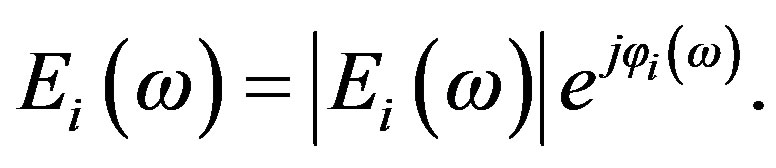 (2)
(2)
Assuming that the transfer function varies slowly around a carrier frequency ωc with constant amplitude and a linear varied phase, then
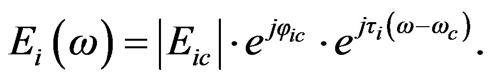 (3)
(3)
Here, the phase is approximated by the first two terms of its Taylor’s series [10]
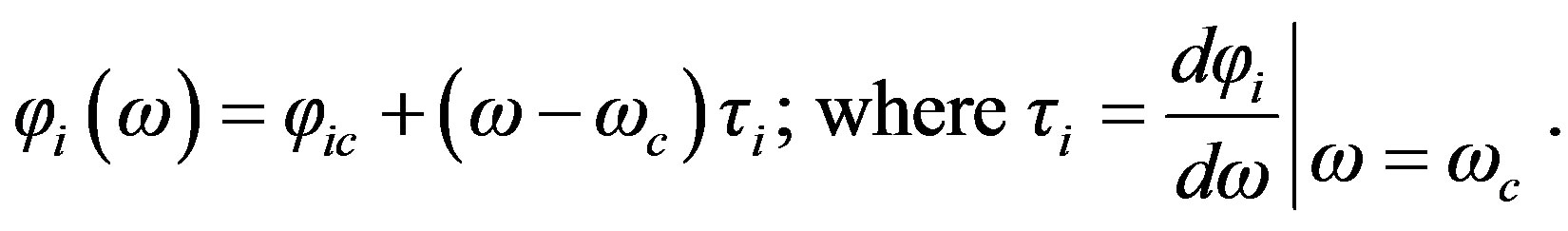 (4)
(4)
jic is the phase of Ei(ω) at ωc, τi is the time delay of propagation of the field along the i path with respect to reference direct path contribution. Eic is a complex parameter that depends on the antenna gain and geometry and also includes the coefficients of coupling mechanism: reflection coefficients, diffraction coefficients etc. The in-phase and quadrature components of the baseband transfer function is [10]
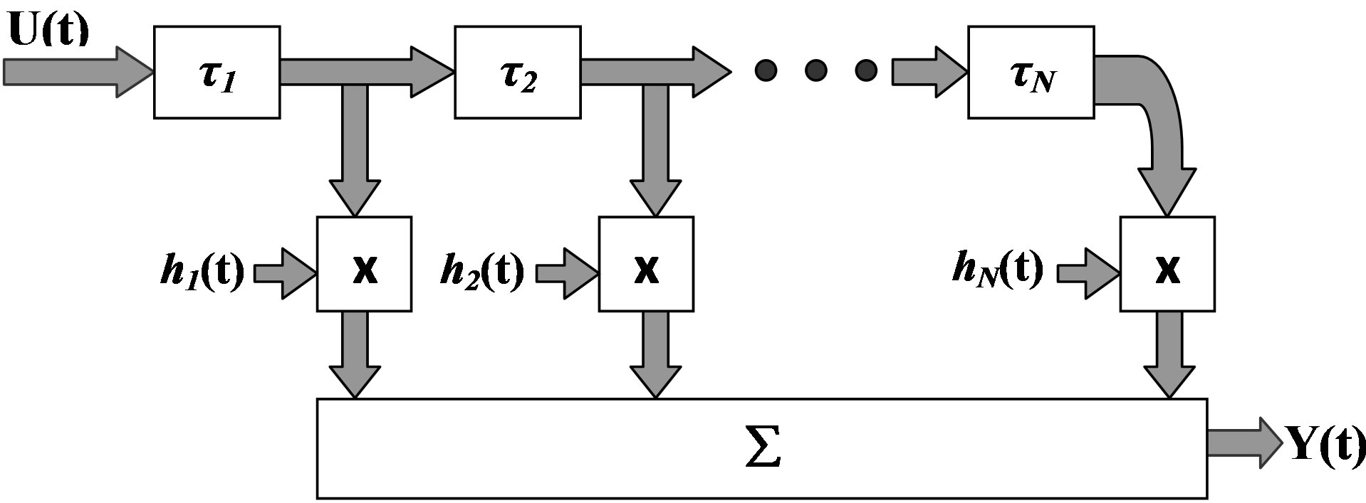
Figure 2. Wideband channel model.
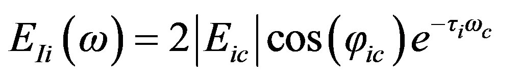 (5)
(5)
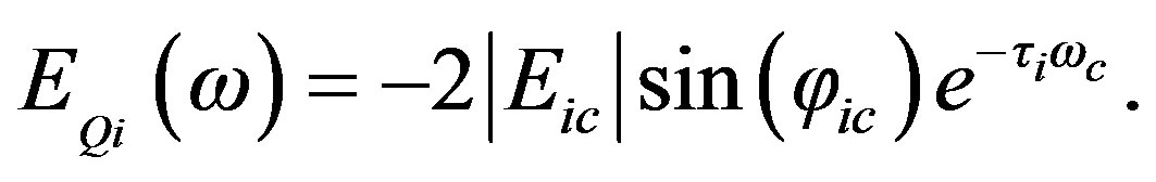 (6)
(6)
Therefore the in-phase and quadrature components of baseband impulse function can be obtained by inverse transform of (5) and (6) as follow
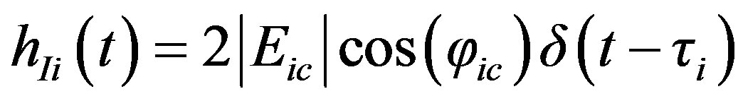 (7)
(7)
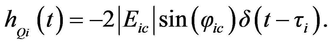 (8)
(8)
The modulus of the baseband impulse response hi(t) for coupling mechanism i will be
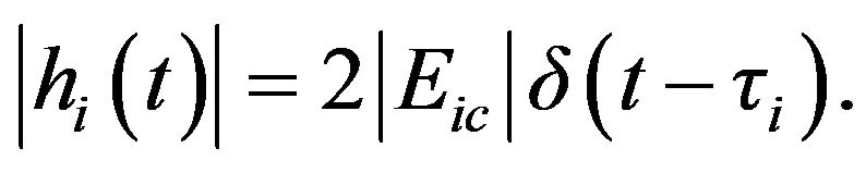 (9)
(9)
From (3), the transfer function of the total electric field is
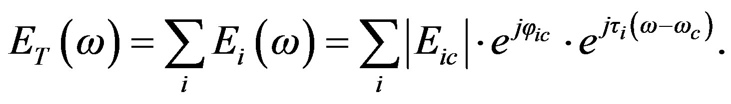 (10)
(10)
From (9), the amplitude of base band impulse response for the whole radio channel is given by
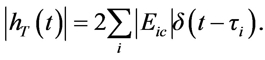 (11)
(11)
To calculate the transfer function and the associated impulse response at certain elevation angle, initially, the model will determine the expected ray contributions at this elevation angle (zone) according to the data listed in Table 1. Figure 3 sketches the expected ray contributions at the zone defined by elevation angles between qRSBBldgMax and 180˚. After that, the model will calculate the transfer function and the impulse response for each ray contribution using (3) and (9). Finally, (10) and (11) will be used to compute the transfer function and the impulse response of the whole channel at the considered elevation angle.
The procedure of calculating the transfer function and impulse response can be exemplified by the first case a in Table 1 for ground reflected and second order diffracted ray shown in Figure 4. As it can be seen in this figure, the incident field at point M corresponds to a direct incident ray; hence it can be considered as a reference
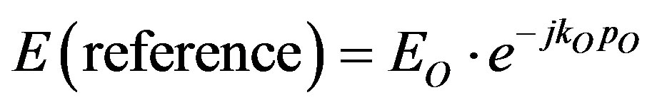 (12)
(12)
where ko= ωc/C is the free space wave number. C is the speed of light. The reflected then second order diffracted field at the mobile can be written as
 (13)
(13)
Γg(.) is the ground reflection coefficient and defined as [11]
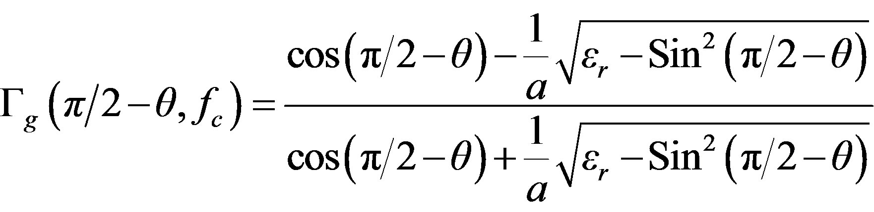 (14)
(14)
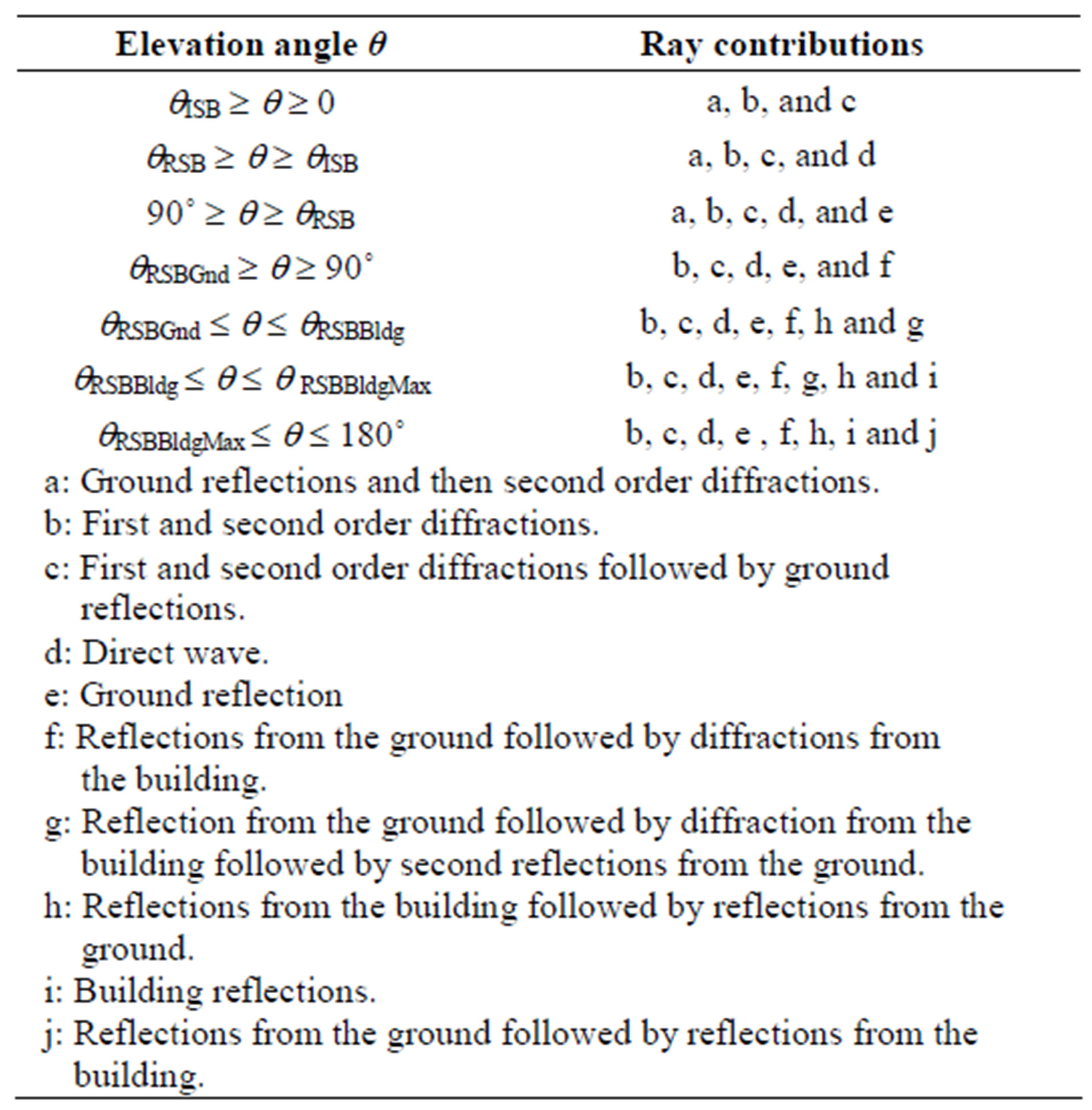
Table 1. Ray contributions at different zones.
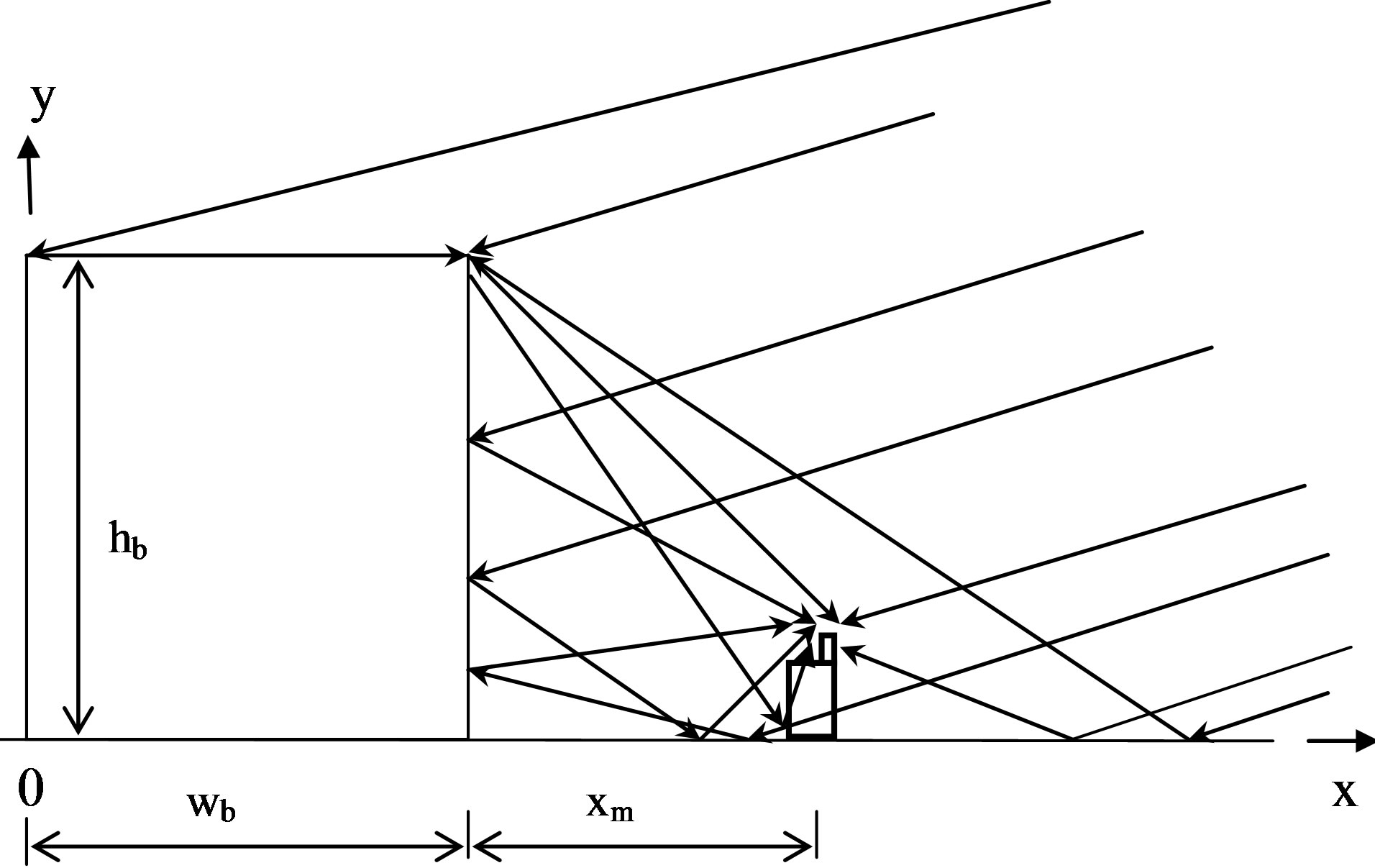
Figure 3. Zone for ray contributions due to building blockage at elevation angle q (qRSBBldgMax £ q £ 180˚).
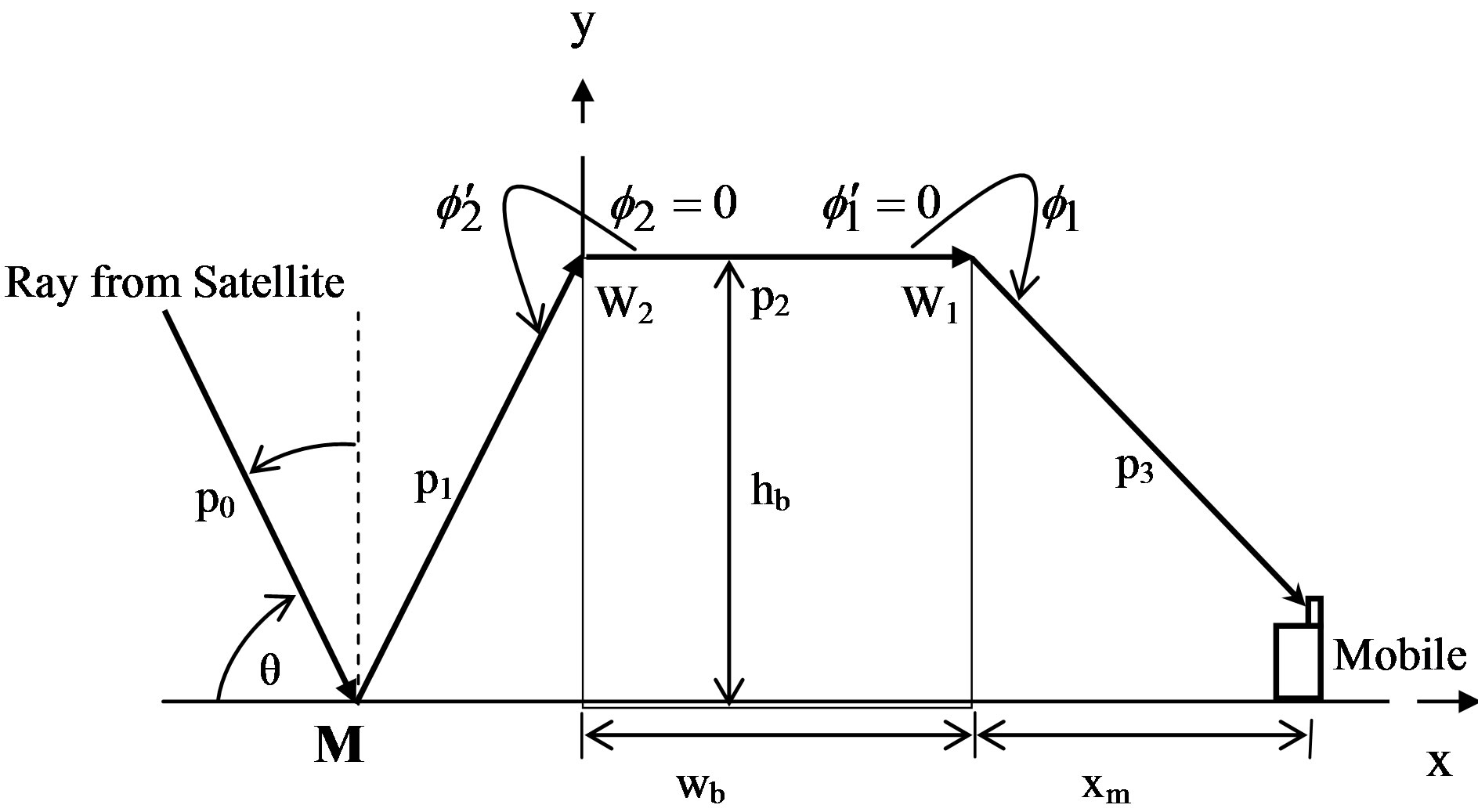
Figure 4. Zones for reflected diffracted ray contribution.
where a = 1 for horizontally polarized incident wave and a = er for vertically polarized incident wave. The ground permittivity er is [11]
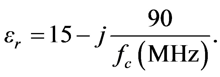 (15)
(15)
The building edge diffraction coefficient is defined as [12]
 (16)
(16)
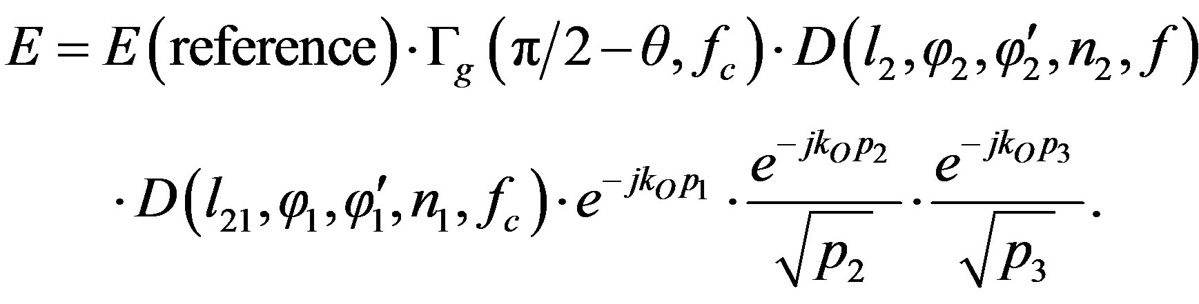
where C is the light speed and fc is the carrier frequency of the diffracted signal. The minus sign between the curly brackets is used for horizontal polarization and plus sign for vertical polarization. L is the distance parameter, n is the wedge index (in our case n = 1.5), and F[koLg± (f ± f')] is the Fresnel transition integral [12]. The field in (13) can be reformulated as
 (17)
(17)
As it can be seen in Figure 4, (p1 + p2 + p3) represent the path difference between the reflected-diffracted ray and the direct one; thus the corresponding time delay t1 = (p1 + p2 + p3)/C. Hence, using (3), the transfer function of this ray contribution will be as follow
 (18)
(18)
The normalized E(ω) with respect to E(reference) is
 (19)
(19)
with amplitude of
 (20)
(20)
Thus the modulus of the baseband impulse response of this ray contribution is then
 (21)
(21)
In terms of the building and mobile dimensions and the distance between them (see Figure 4), p1, p2, p3, f1, f2,  ,
,  , L2 and L21 can be defined as
The same procedure can be applied to derive the transfer function and impulse response for other ray contributions in terms of the geometrical dimensions and the elevation angle.
3.2. Power Delay Profile
The power delay profile (PDP) is defined as the variation of mean power in the channel with delay [9], thus the mean power of signal ray contribution of delay τi can be defined as
 (21)
(21)
where E[.] is the mean square value of the amplitude of time variant impulse response hi(t). Usually the PDP is discretized in the delay dimension to yield n individual taps of power P1, P2, ,Pn. Each tap-gain process may be Rice or Rayleigh distributed [5]. The PDP can be characterized by various parameters:
● Maximum excess delay (t–10 dB): The maximum delay for a multipath component within –10 dB of the strongest arriving multipath signal.
● Mean delay: the delay corresponding to the “center of gravity” of the profile; defined by
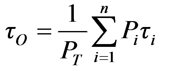 (22)
(22)
where the total power is
 (23)
(23)
● Root-Mean-Square delay (trms): the second moment, or spread, of the taps which takes into account the relative power of the taps as well as delay
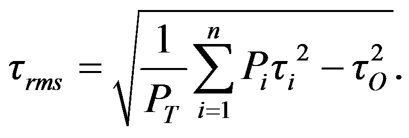 (24)
(24)
This makes  a better indicator of system performance than the other parameters. Since it can be considered as an indicator of the system error rate performance for moderate delay spread (within one symbol duration).
4. Results
A matlab program has been written to calculate the channel transfer function, the impulse response and the power delay profile including its delay parameters (to, t–10 dB and trms). Figures 5-8 show the channel transfer function for different elevation angles and at different environments (residential and urban) for vertically polarized signal. The shadow boundary qISB for residential building of 14 m height and 10 m width at a distance of 20 m away from the building is 47.7˚. In the first case of Figure 5 with q < qISB, the received signal is mainly affected by shadowing effect (no direct signal), which can also be observed from the small amplitude. In the other case of Figure 6 at q > qISB there are money unblocked signal contributions that increase the signal level. The interaction between these maultipath signals of different delays results in considerable variation of the amplitude
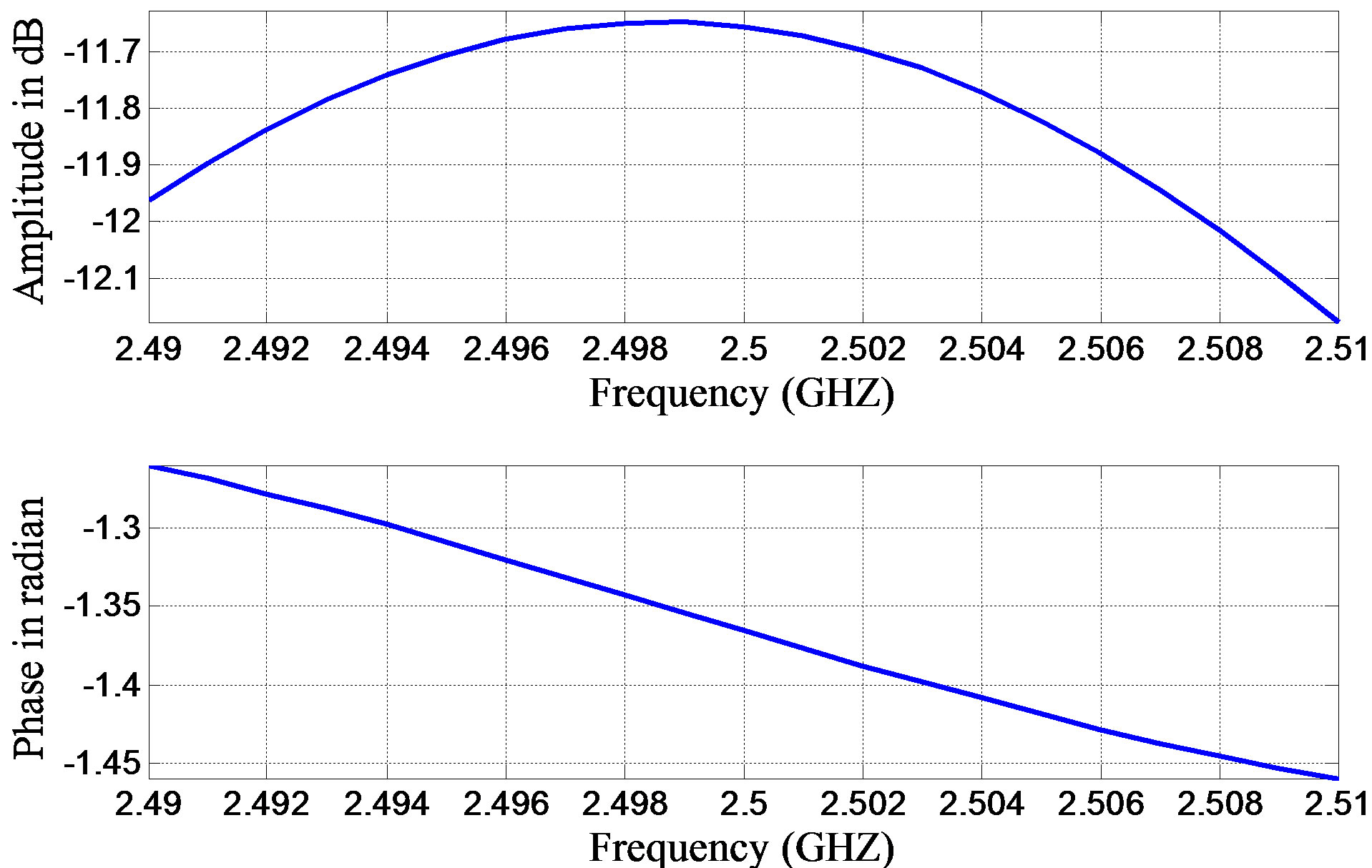
Figure 5. LMS channel transfer function at 45˚ elevation angle for 14 m building height and 10 m building width at a distance of 10 m away from the building in residential area.
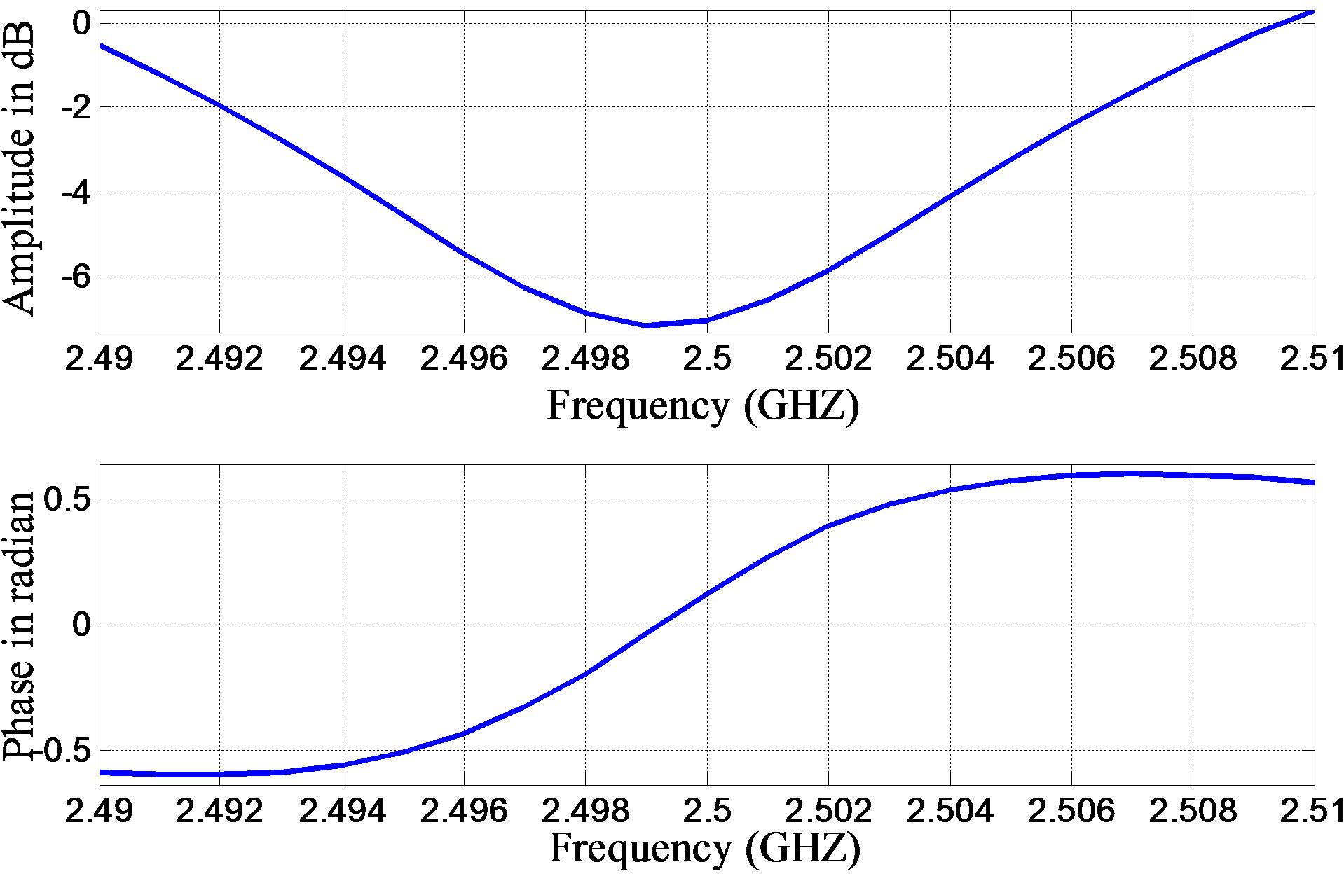
Figure 6. LMS channel transfer function at 90˚ elevation angle for 14 m building height and 10 m building width at a distance of 10 m away from the building in residential area.
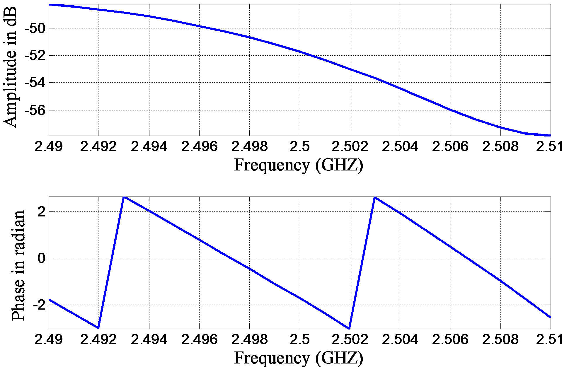
Figure 7. LMS channel transfer function at 45˚ elevation angle for 112 m building height and 20 m building width at a distance of 10 m away from the building in urban area.
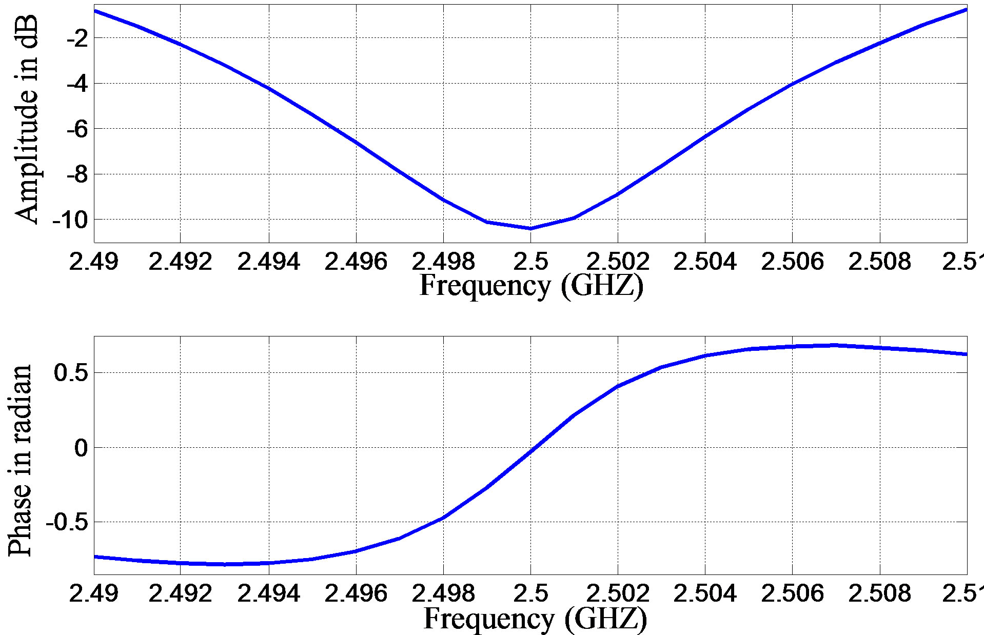
Figure 8. LMS channel transfer function at 90˚ elevation angle for 112 m building height and 20 m building width at a distance of 10 m away from the building in urban area.
of the transfer function around the carrier frequency 2.5 MHz. The –6 dB bandwidth in this case is around 17 MHz. The shadow boundary qISB for urban building of 112 m height and 20 m width at a distance of 10 m away from the building is 84.7˚. In the first case of Figure 7 with q < qISB, the received signal is also affected mainly by shadowing effect, which can also be observed from the smaller magnitude of the transfer function.
In the other case of Figure 8 of q > qISB the received signal is significantly faded due to stronger maultipath mechanism, which can also observed for the smaller amplitude around the carrier frequency 2.5 MHz. The –6 dB bandwidth in this case is around 12.5 MHz. With respect to the last case of Figure 6, of the same elevation angle, the expected deterioration (amplitude variation and the associated frequency selectivity effect) of the radio channel as the mobile is moved from residential to urban environment has been predicted by the model.
Tables 2-5 present calculation results for the mean values of to, t–10 dB, and trms in urban and residential environments for line-of-sight (LOS) of q > qISB and out-of-sight (OOS)
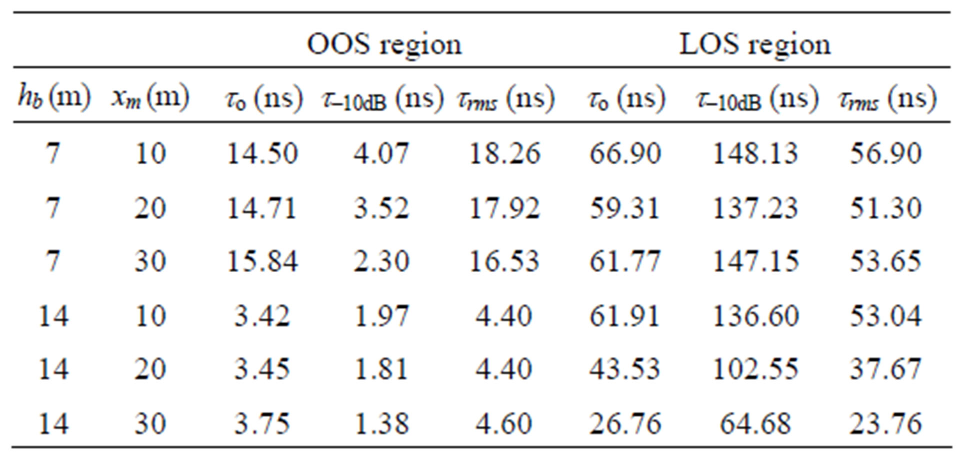
Table 2. Time delay parameters for residential environment.
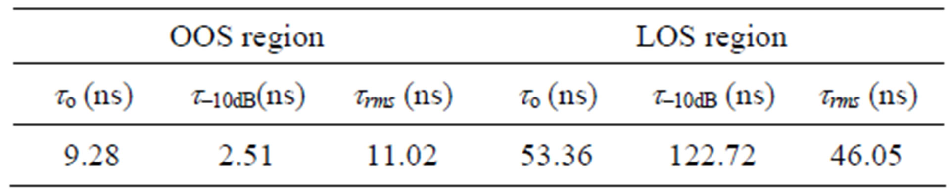
Table 3. Mean time delay for residential environment.
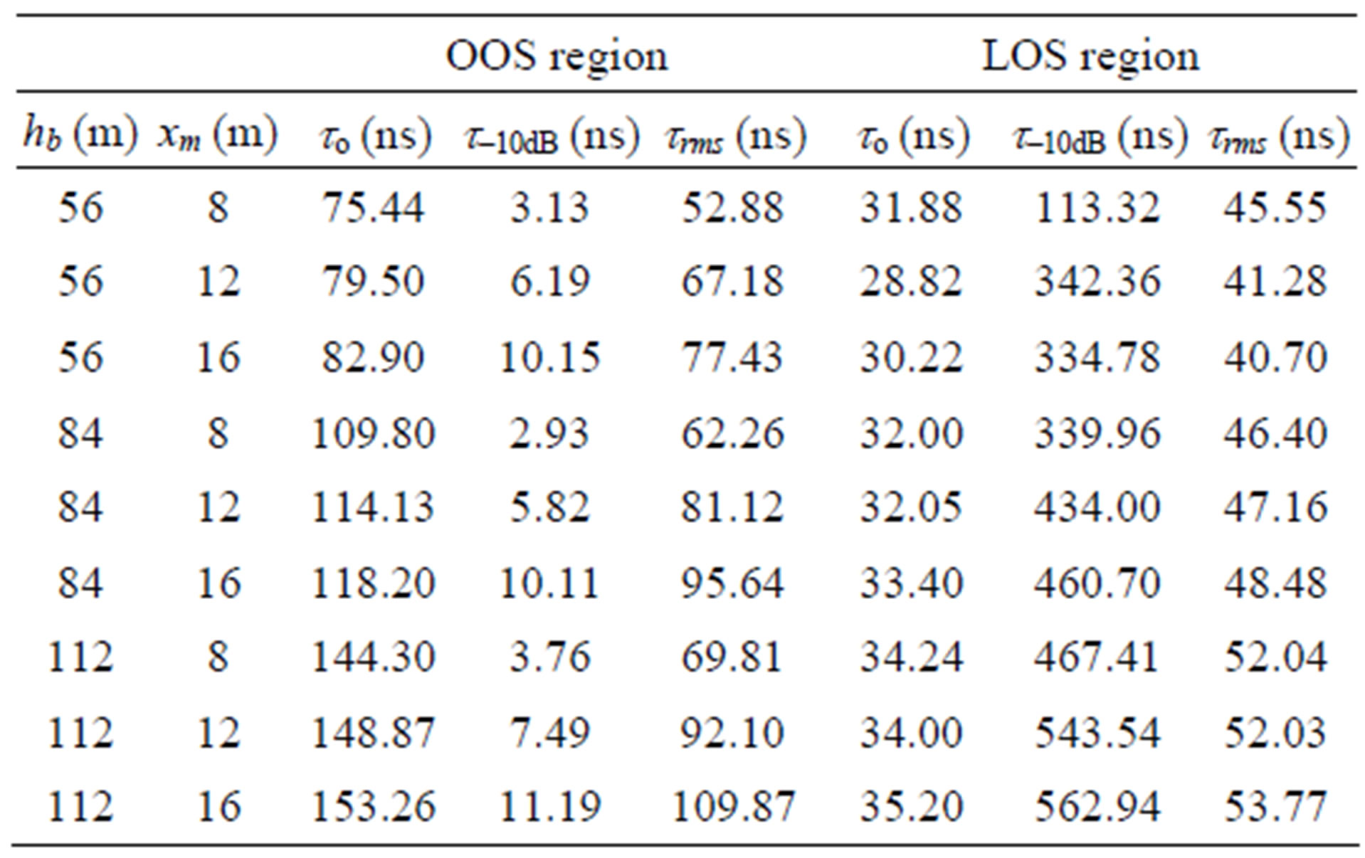
Table 4. Time delay parameters for urban environment.

Table 5. Mean time delay for urban environment.
of q < qISB zones. As it can be seen in Table 2 and 4, higher values for to and trms can be observed in the OOS zone, and thus stronger signal distortion (time spreading) is predicted especially in the urban. In this zone also t–10dB has smaller values due to the stronger attenuation for the signal ray contributions. In the LOS zone, there is smaller variation for the signals delays in the residential areas and it can be reduced by moving the mobile far away from the building (to and trms decrease by increaseing xm). In urban environments to and trms are affected mainly by the building height and therefore standing away from the building may not provide significant improvement for the received signal at the mobile.
Tables 3 and 5 show comparable value for the mean of trms in both urban and residential environments. This can be related to scaling of the value of this parameter by
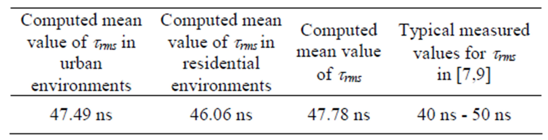
Table 6. Comparison between computed and measured trms.
the received power. In urban area, the value of time delay is larger but the received power is smaller. On the other hand, in residential environment, the value of time delay is small but the received power is larger. Table 6 compares the simulated and measured trms. The mean value of computed trms is equal to 47.78 ns and this value is in the range of typical values for mobile satellite (40 - 50 ns) reported in [7] and [9].
5. Conclusion
A wideband propagation model for LMS radio channel has been derived and implemented in Matlab software. The model has been used to calculate the received signal at the mobile for different satellite elevation angles and also in different environments (residential and urban). The simulation results showed that the frequency selectivity effect increases as one moves from residential to urban environment; and therefore this accordingly limits the usable transmission bandwidth. Also the power delay profile analysis showed that the time spreading effect, which can be used as an indication for the rate of ISI of the LMS, increases in the urban areas with respect to residential ones. The obtained values for the time delay, using the developed model, have a good agreement with measured ones in other published papers.
REFERENCES
- G. Maral and M. Bousquet, “Satellite Communicant Systems,” 3rd Edition, Wiley, New York, 2000.
- C. Loo, “A Statistical Model for Land Mobile Satellite Link,” IEEE Transactions on Vehicular Technology, Vol. 34, No. 17, 1985, pp. 122-127.
- M. Dottling, A. Jahn, D. Didascalou and W. Wiesbeck, “Twoand Three Dimensional Ray Tracing Applied to the Land Mobile Satellite (LMS) Propagation Channel,” IEEE Antenna and Propagation Magazine, Vol. 43, No. 6, 2001, pp. 27-37. doi:10.1109/74.979492
- S. Saunders, C. Tzaras and B. Evans, “Physical-Statistical Methods for Determining State Transition Probabilities in Mobile-Satellite Channel Models,” International Journal of Satellite Communications, Vol. No. 3, 2001, pp. 207- 222.
- M. S. Al Salameh and A. H. Jarndal, “Impact of Buildings on the Performance of MEO Satellite Mobile Communication System for Low Bit Rate Application,” IEE Proceedings on Microwaves, Antennas and Propagation, Vol. 151, No. 2, 2004, pp. 161-166. doi:10.1049/ip-map:20040149
- M. S. Al Salameh and S. A.-R. T. Mahmoud, “MoM Solutions to Building Blockage of Mobile Satellite Communications,” International Journal of Electronics, Vol. 98, No. 12, 2011, pp. 1639-1658. doi:10.1080/00207217.2011.609974
- B. Belloul, S. R. Saunders, M. A. Parks and B. G. Evans, ”Measurement and Modeling of Wideband Propagation at L-Band and S-Bands Applicable to the LMS Channel,” IEE Proceedings on Microwaves, Antennas and Propagation, Vol. 147, No. 2, 2000, pp. 116-121. doi:10.1049/ip-map:20000220
- C. Oestges, H. Vasseur and D. Vanhoenacker, “Impact of Edge Diffraction on Performance of Land Mobile Satellite System in Urban Areas,” 28th European Microwave Conference, Amsterdam, October 1998, pp. 357-361. doi:10.1109/EUMA.1998.338178
- S. R. Saunders, “Antenna and Propagation for Wireless Communication Systems,” John Wiley & Sons, Chichester, 1999.
- M. F. Catedra and J. Perez-Arriaga, “Cell Planning for Wireless Communications,” Artech House, London, 1999.
- S. Ramo, J. R. Whinnery and T. V. Duzer, “Fields and Waves in Communication Electronics,” John Wiley, New York, 1994.
- A. C. A. Balanis, “Advanced Engineering Electromagnetics,” Wiley, New York, 1989.