Journal of Electromagnetic Analysis and Applications
Vol. 3 No. 9 (2011) , Article ID: 7452 , 8 pages DOI:10.4236/jemaa.2011.39055
New Formula for Evaluating the Number of Unit Cell of a Finite Periodic Structure Considered as Infinite Periodic One
![]()
SYSCOM Laboratory, Department of Information and Communications Technology, National Engineering School of Tunis, Tunis, Tunisia.
Email: bouali_samia@yahoo.fr
Received June 22nd, 2011; revised July 24th, 2011; accepted August 7th, 2011.
Keywords: Periodic Structure, Floquet Theorem, Dispersion Relation, Scattering Parameters, Input Impedance
ABSTRACT
This paper presents a modeling and an analysis of one-dimensional periodic structure composed of a cascade connection of N cells considered as infinite. The ABCD matrix representations with the Floquet analysis have been used to derive the dispersion relation and input impedance of infinite periodic structure. The transmission matrix for the N identical cascaded cells has been successfully used to obtain an efficient and easy-to-use formula giving the necessary number of cells such that they can be considered infinite. As an illustrative example, the formula is applied and verified to finite size TL periodically loaded with obstacles. Scattering parameters and the input impedance of the structure are expressed and plotted.
1. Introduction
A periodic structure consists fundamentally of a number of identical structural components “periodic elements” which are joined together end to end or side by side to form the whole structure [1,2]. In fact, periodic structures are investigated in several applications in the electromagnetic engineering. For instance, these structures can be used to design frequency-selective surfaces [4], photonic crystals [5-8], and meta-materials [9]. Hence periodic structures have become a field of intense research activities. If the periodic structure is an infinite array, simple methods based on the Floquet’s theorem [1] or the periodic Green’s function [10], can be applied, where the characterization of the whole periodic structure can be reduced to the analysis of only a single cell. However, the infinite periodic structure is a theoretical case because in actual applications all periodic structures have finite size. Hence, the accurate analysis of the finite periodic structures usually needs to solve a large-scale problem. There are various methods to analyze finite periodic structures such as the finite-difference timedomain (FDTD) method [11], the moment method MoM [12], the subentire-domain (SED) basis functions and the conjugate-gradient fast Fourier transform (CG-FFT) [13, 14].
In this paper, we investigate the various characteristics of finite and infinite (1-D) periodic structure by microwave techniques. The study of the infinite periodic structure is reduced to a single unit cell, Floquet theorem is invoked and both dispersion diagram and input impedance are obtained. For the case of finite periodic structure we suppose that a finite structure with a very large number of unit cell, can be considered as an infinite structure, using the transmission matrix for the N identical cascaded cells, a condition of convergence of the finite structure to an infinite structure is concluded. This convergence condition helps to find the minimal number of unit cell necessary such that they can be considered infinite. The accuracy and the efficiency of the proposed formula was verified to a finite size TL periodically loaded with obstacles, a scattering matrix analysis have applied input impedance and S parameters are calculated and plotted. Dispersion diagram, the stop and pass band property, the effect of changing geometrical parameters on the pass (stop) bandwidth, attenuation and phase constant are shown.
2. Periodic Structure Model
The periodic structure discussed in this paper is made of an infinite or finite repetition of a unit cell in one dimension. Each unit cell of this structure is characterized by its matrix chain; the study of the infinite periodic structure is reduced to a single unit cell as shown in Figure 1; we use the ABCD matrix with the Floquet analysis to model the infinite structure.
2.1. The Infinite Periodic Structure
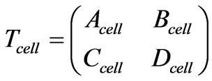
The foundations of periodic structure theory are developed in [2] and [3], these references show that a periodic structure supports pure progressive waves propagating toward +Z or –Z, usually referred to as Bloch waves. If a unit cell in the structure is defined by its transmission matrix Tcell (the so-called ABCD matrix witch parameters named Acell, Bcell, Ccell, and Dcell), we can write the matrix of the unit cell
 (1)
(1)
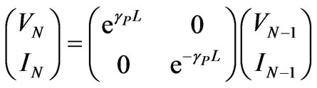
The input impedance of the infinite structure Zin can be found by modeling the structure as shown in Figure 1. According to the Floquet’s theorem for infinite periodic structures [1-3], the input and output relationship of the nth unit cell are given by:
 (2)
(2)
The parameters VN and IN are voltage and current corresponding to the propagating wave threw the nth unit cell.
 (3)
(3)
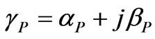
The parameter  is the complex propagation constant of the periodic structure (where αp is the attenuation constant and βP is the phase constant) and L is the period of the structure shown in Figure 1
 (4)
(4)
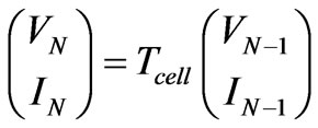
Equations (2) and (4) give:
 (5)
(5)
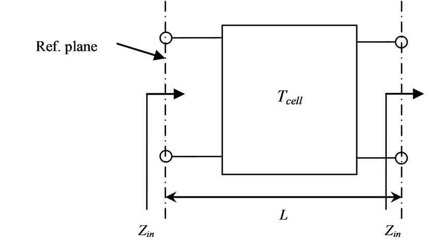
Figure 1. Unit cell of periodic structure.
The resolution of (5) gives the dispersion relation. The input impedance of the structure is given by the resolution of (6)
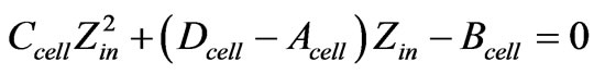 (6)
(6)
2.2. The Finite Periodic Structure
By using Floquet analysis of an infinite periodic structure the feature of the overall system can be extracted by considering one single unit cell [2]. In practice the number of unit cell is always limited, so an infinite periodic structure is a theoretical case, we propose to determinate the number of unit cells permitting that several aspects of a finite periodic structure demonstrate the same behavior of an infinite periodic structure.
We consider a simple finite structure that is periodic in one dimension. The structure can be modeled by cascading its transmission matrix with two boundaries at the beginning and the end of the structure, as illustrated in Figure 2.
The unit cell of the periodic structure is considered reciprocal; its transmission matrix is given by (1), its determinant is equal to 1 (det(Tcell) = 1).
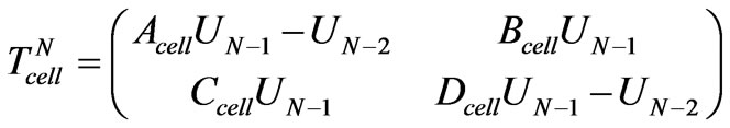
The transmission matrix of the N identical cascaded cells is given by:
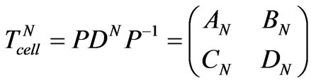 (7)
(7)
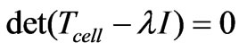
D is the diagonal matrix formed by the eigenvalues of the matrix Tcell, P is a matrix consisting of the eigenvectors corresponding to the eigenvalues in D. The eigenvalues of Tcell are λ and µ which are given by:
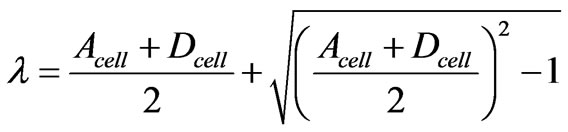 (8)
(8)
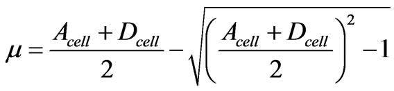 (9)
(9)
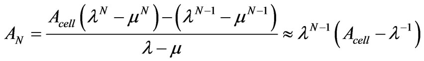
By cascading N unit cell the matrix chains of the total structure can be written according to λ or µ.
 (10)
(10)
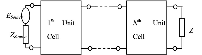
Figure 2. Finite periodic structure in microwave circuits.
The overall transmission matrix can also be written as [15]:
 (11)
(11)
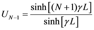 (12)
(12)
 (13)
(13)
The S parameters S11 and S21 associated with the entire structure shown in Figure 2 are expressed by:
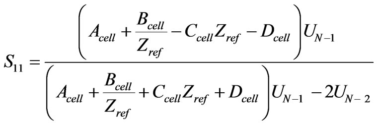 (14)
(14)
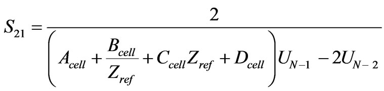 (15)
(15)
Zref is reference impedance which is usually chosen 50 Ω and UN–1 is a parameter defined by (12).
The input impedance of such a structure can be found in different ways. One way is to start from the last segment finding its input impedance which is the load impedance for the former segment and repeat the same procedure until the end. In addition, in ABCD matrix representation [2] the input impedance is:
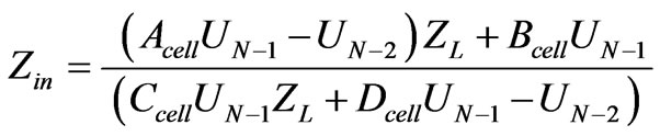 (16)
(16)
2.3. Evaluation of the Number of Unit Cells
In the context of infinite periodic structure (infinite number of unit cells), both floquet theorem and continuous dispersion curve are usually used. For finite periodic structure (finite number of unit cells) and by raising the number of unit cells at the convergence we must have the same results as the case of infinite periodic structure. In this section we propose to find this finite number of unit cells which allow to show the same result as the infinite case.
We have if │λ│> 1 then 0 <│µ│ < 1 and vice versa. If N is very large and tends towards the infinite then by using (10) we have:
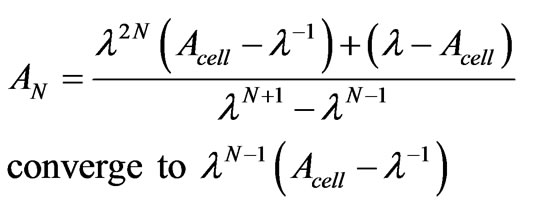 (17)
(17)
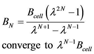 (18)
(18)
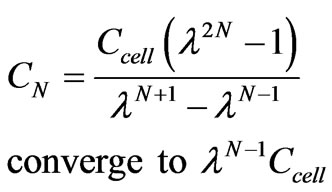 (19)
(19)
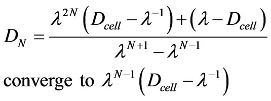 (20)
(20)
When N is very large the structure is considered infinite, we propose to find the value of N from which finished structure is equivalent to an infinite structure. By using (17) we can write if N very large then:
 (21)
(21)
By developing this equality we obtain:
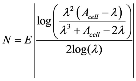 (22)
(22)
with E(x) is the integer part of x.
N is the number of cells necessary to consider the finite structure as an infinite one. It’s depending on the physical characteristic of the unit cell Acell and Dcell. For any finite periodic structure modeled by scattering matrix we can determinate the sufficient number of unit cell to approach the infinite case, then by using this finite number we can approach easily the infinite case.
Dispersion diagram contains information regarding the wave properties of the structure and input impedance reflects properties of the structure from circuit point of view which depend on the cell parameters. For this reason another way to find the number of cells necessary such that structure can be considered infinite, is to start from finite structure in Figure 3 with 2 unit cells then we compare between Zin of the finite and infinite structure and continues to the convergence criteria. The algorithm displayed in Figure 3 describes the procedure of this method.
Convergence is considered to be reached if the difference between the input impedance of finite and infinite structure is less than 0.01%.
3. Numerical Results and Discussion
In order to verify the accuracy and efficiency of the proposed formula, we consider a finite-size TL periodically loaded with obstacles and constituted by the repetition of N unit cell. A unit cell is considered as a three part network one half (L/2) of the transmission line, the loading element JX and another half (L/2) of the transmission line as shown in Figure 4.
Therefore, the matrix of the unit cell can be obtained by cascading three matrix:
• First, the matrix of the half (L/2) of the transmission line.
• Second, the matrix of the element JX.
• Third, the matrix of the half (L/2) of the transmission line.
The transmission matrix of the half (L/2) of the transmission line is given by:
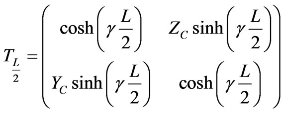 (23)
(23)
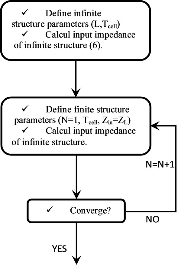
Figure 3. Determination of the number of cells necessary to have an infinite structure.
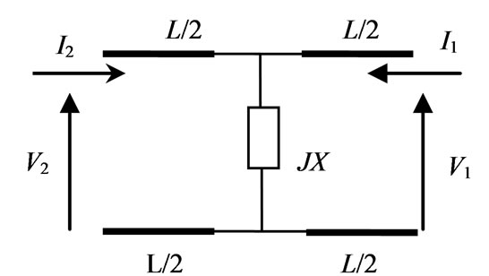
Figure 4. Schema of the unit cell.
where γ the transmission line propagation constant, L is the length of the transmission line and Zc is the transmission line characteristic impedance.
The transmission matrix of the element JX lumped shunt admittance is given by:
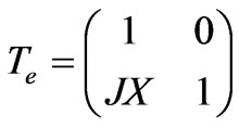 (24)
(24)
The matrix of the unit cell is given by:
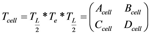 (25)
(25)
 (26)
(26)
3.1. The Infinite Periodic Structure
In the lossless case we have
 (27)
(27)
In this case, we use (5), (26) and (27) to define the dispersion relation of this structure as follows:
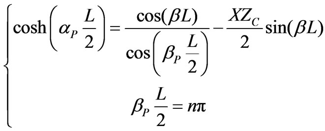 (28)
(28)
 (29)
(29)
To simplify theses equations we pose:
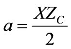 (30)
(30)
and
 (31)
(31)
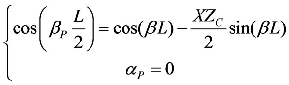
Using (28) and (29), the attenuation and phase constant can be written as:
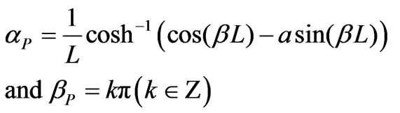 (32)
(32)
 (33)
(33)
If a cell is reciprocal and symmetrical, the input impedance of the infinite structure is:
 (34)
(34)
In (28) the attenuation constant  is varying and the phase constant
  is fixed. For this equation if
the periodic structure supports a propagation waves, else
no wave can propagate along the periodic structure.
In (29) the attenuation constant  and the phase constant
  is varying. For this equation if
is varying between –1 and +1, the periodic structure supports a non attenuated propagation waves. Else no wave can propagate along the periodic structure. The dispersion diagram is depicted in Figure 5 and Figure 6 for different parameters of the structure.
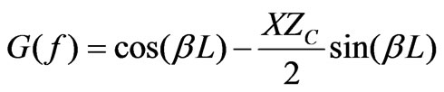
To simulate the structure we can vary two parameters: the parameter (a = XZ/2) or the length of the unit cell (L). We present the results for several cases by varying (a) and L. The dispersion curve with attenuation is obtained by plotting G(f), the frequency ranges corresponding to G(f) larger than 1 indicate the pass band while the frequency regions with G(f) < 1 correspond to the stop band. For the dispersion curve without attenuation to have propagation G(f) should be between –1 and +1. The attenuation and phase constants were calculated and plotted. Simulations results show the presence of stop band and pass band. The attenuation and phase constants were calculated by using the two equations of dispersion. This agrees well with the stop and pass bands. The frequency ranges corresponding to the stop and pass
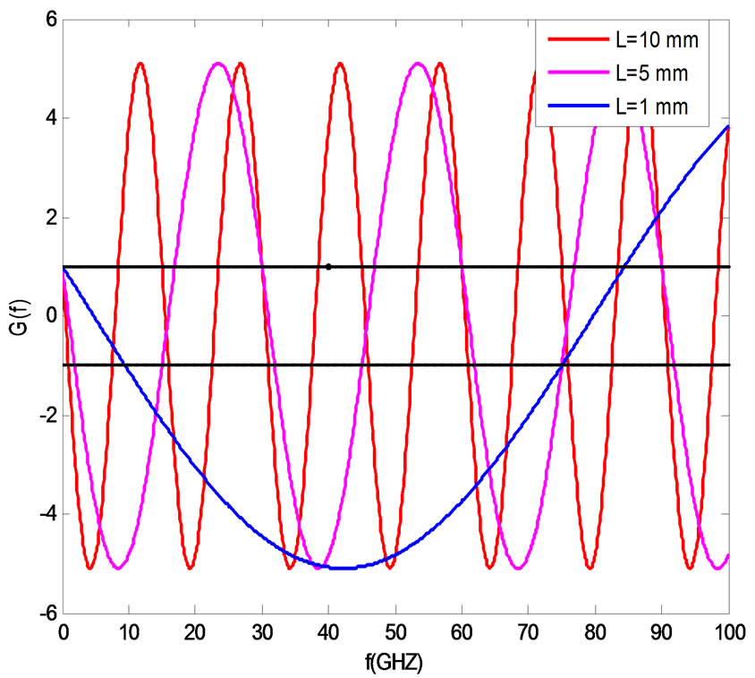
Figure 5. Dispersion Diagram for three values of L and a = 5.
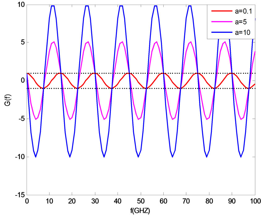
Figure 6. Dispersion Diagram for three values of a and L = 10 mm.
band depend on the physical configuration of the periodic structure (L) and the obstacle (JX).
The range of the frequency in Figure 5 (respectively Figure 6) represents propagation without attenuation agree well with Figure 7 (respectively Figure 8) that we have α = 0 and Figure 9 (respectively Figure 10) that we have β ≠ 0 it’s a non attenuated propagation (α = 0 and β ≠ 0). The range of the frequency in Figure 5 represents propagation with attenuation agree well with Figure 7 that we have α ≠ 0 and Figure 9 that we have β = 0 it’s an attenuated wave.
3.2. The Finite Periodic Structure
Using (22), we obtain N = 12 as a sufficient value to approach the infinite case. In order to verify this value we
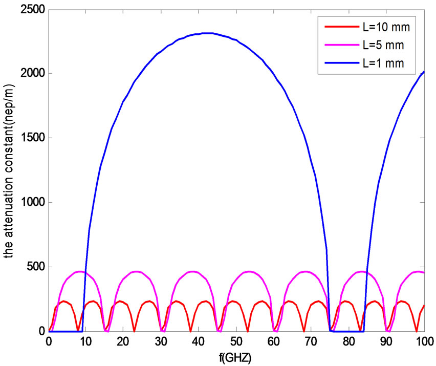
Figure 7. The attenuation constant for three values of L,
a = 5.
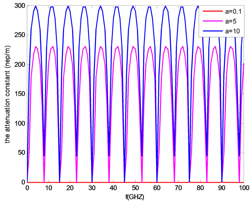
Figure 8. The attenuation constant, for three values of a, L = 10 mm.
have plotted the input impedance of the structure for several value of N (10, 12 and infinite).The examination of the curves on the various frequency bands show that the input impedance of the 12 unit cell has an excellent agreement with the input impedance of the infinite structure. The variation of input impedance (absolute value) over frequency for finite (N = 10, 12) structure is illustrated in Figure 11 and Figure 12 by iterative method (Figure 3). The input impedance based on finite periodic structure is shown in this graph for number of unit cells of N = 10 and 12. It is seen that the input impedance reaches the limit of infinite periodic structure, if the number of unit cells are in order of 12.
It is clearly observed that the input impedance of finite structure reaches the limit of corresponding infinite case,
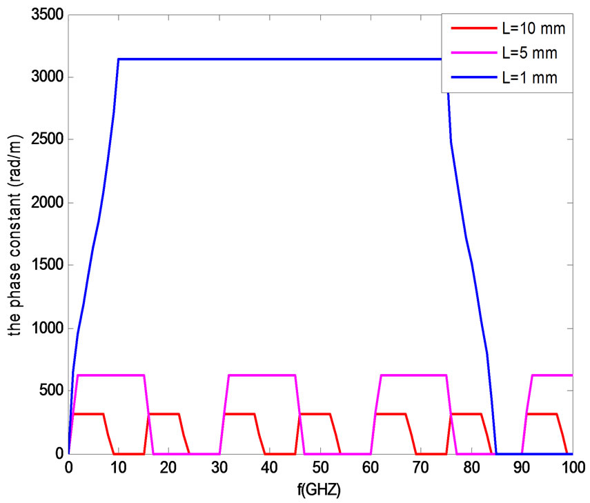
Figure 9. The phase constant, for three values of L, a = 5.
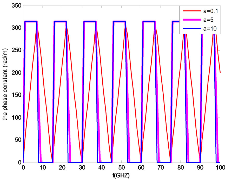
Figure 10. The phase constant, for three values of a, L = 10 mm.
if the number of unit cells is in order of 12.
The input impedance of a finite periodic structure is depicted in Figure 13 by using ABCD matrix method (16), we put the load of ZL= 50 Ω.
By increasing the number of unit cells, the number of fluctuations will also increase which is illustrated in Figure 13.
In order to compare those results to those from scattering parameter calculation, the scattering parameters are displayed in Figure 14. They are calculated based on (14) and (15).
4. Conclusions
Infinite and finite periodic structures have been investigated. In the case of infinite structure, the Floquet theorem has been invoked, and both dispersion diagram and
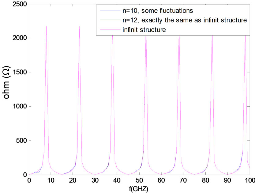
Figure 11. Input impedance for the case of infinite and finite unit cells a = 10 and L = 10 mm.
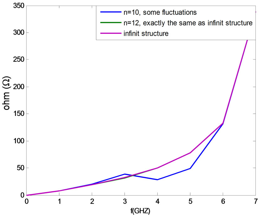
Figure 12. Input impedance in the case of infinite and finite unit cells (a = 10 and L = 10 mm).
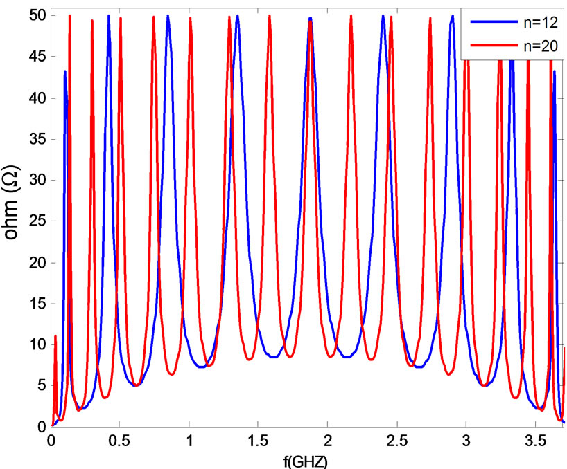
Figure 13. Input impedance for the finite structure (a = 1, L = 10 mm, ZL = 50 Ω).
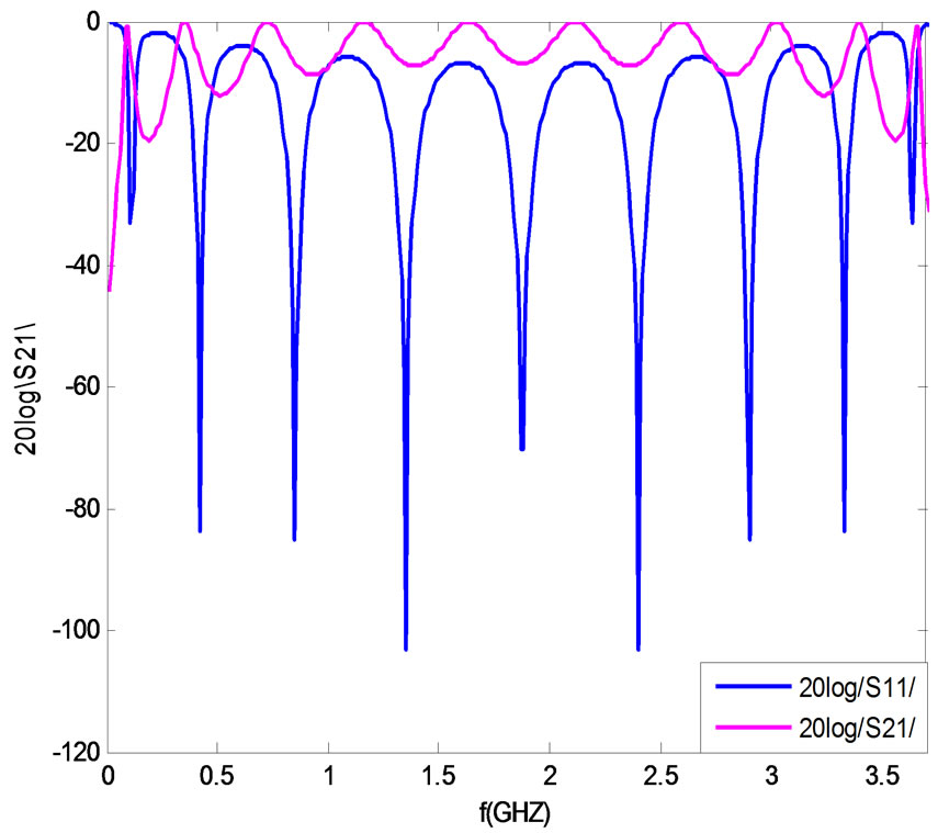
Figure 14. S-parameters for the finite periodic structure N = 12, Zref = 50 Ω.
input impedance have been obtained. By using scattering matrix and applying boundary conditions for the case of finite structure, both input impedance and S-parameters have been obtained and an efficient and easy-to-use formula to find the necessary number of unit cell for periodic finite structure to be equivalent of an infinite periodic structure has been presented. The formula is verified on a transmission line periodically loaded with obstacles. Simulation results have validated the proposed numerical modeling formula.
REFERENCES
- L. Brillouin, “Wave Propagation in Periodic Structures,” Dover, New York, 1953.
- R. Collin, “Foundations for Microwave Engineering,” 2nd Edition, Wiley-IEEE Press, Hoboken, 2000.
- D. Pozar, “Microwave Engineering,” Addison-Wesley, Reading, 1990.
- D. J. Mead, “Wave Propagation in Continuous Periodic Structures: Research Contribution from Southampton 1964-1995,” Journal of Sound and Vibration, Vol. 190, No. 3, 1996, pp. 495-524.
- B. A. Munk, “Frequency Selective Surfaces: Theory and Design,” Wiley, New York, 2000.
- E. Yablonovitch, “Inhibited Spontaneous Emission in Solid-State Physics and Electronics,” Physical Review Letters, Vol. 58, No. 20, 1987, pp. 2059-2062.
- Y. Rahmat-Samii and H. Mosallaei, “Electromagnetic Band-Gap Structures: Classification, Characterization, and Applications,” 11th International Conference on Antennas and Propagation, Manchester, 17-20 April 2001, pp. 560-564.
- J. D. Joannopoulos, et al., “Photonic Crystals: Molding the Flow of Light,” 2nd Edition, Princeton University Press, Princeton, 2008.
- C. Caloz and T. Itoh, “Electromagnetic Metamaterials: Transmission Line Theory and Microwave Applications,” John Wiley & Sons, Inc., Hoboken, 2006.
- K. Yasumoto and K. Yoshitomi, “Efficient Calculation of Lattice Sums for Free-Space Periodic Green’s Function,” IEEE Transactions on Antennas and Propagation, Vol. 47, No. 6, 1999, pp. 1050-1055.
- P. Harms, R. Mittra and W. Ko, “Implementation of the Periodic Boundary Condition in the Finite-Difference Time-Domain Algorithm for FSS Structures,” IEEE Transactions on Antennas and Propagation, Vol. 42, No. 9, 1994, pp. 1317-1324. doi:10.1109/8.318653
- V. V. S. Prakash and R. Mittra, “Characteristic Basis Function Method: A New Technique for Efficient Solution of Method of Moments Matrix Equations,” Microwave and Optical Technology Letters, Vol. 36, No. 2, 2003, pp. 95-100. doi:10.1002/mop.10685
- T. J. Cui, W. B. Lu, Z. G. Qian, X. X. Yin and W. Hong, “Accurate Analysis of Large-Scale Periodic Structures Using an Efficient Sub-Entire-Domain Basis Function Method,” IEEE Transactions on Antennas and Propagation, Vol. 52, No. 11, 2004, pp. 3078-3085.
- W. B. Lu, T. J. Cui, Z. G. Qian, X. X. Yin and W. Hong, “Fast Algorithms for large-Scale Periodic Structures,” IEEE Antennas and Propagation Society International Symposium, Monterey, 20-25 June 2004, pp. 4463-4466.
- P. Yeh, “Optical Waves in Layered Media,” John Willey and Sons Inc., Hoboken, 1988.