Journal of Electromagnetic Analysis and Applications
Vol. 1 No. 1 (2009) , Article ID: 188 , 5 pages DOI:10.4236/jemaa.2009.11001
Analysis of the Magnetic Flux Density, the Magnetic Force and the Torque in a 3D Brushless DC Motor
1Isfahan University of Technology, Isfahan, Iran.
Email: majidpakdel@yahoo.com
Received January 8th, 2009; revised February 4th, 2009; accepted February 18th, 2009.
Keywords: Brushless DC Motor, Finite Element Analysis, Maxwell 3 D V 11.1
ABSTRACT
As permanent magnet motors and generators produce torque, vibration occurs through the small air gap due to the alternating magnetic forces created by the rotating permanent magnets and the current switching of the coils. The magnetic force can be calculated from the flux density by finite element methods and the Maxwell stress tensor in cylindrical coordinates. In this paper the magnetic flux density, the magnetic force and the torque of a real three dimensional brushless DC motor are simulated using Maxwell 3 D V 11.1.
1. Introduction
Magnetic force analysis is important in determining not only the torque as the output of motor, but also the source of vibration in machine itself. Vibration is induced in permanent magnet DC motors and generators as shown in Figure 1, by traveling magnetic forces. Neodymium and other rare earths have greater retentivity, coercive force and maximum energy product than traditional ferrite magnets. Therefore, since the magnetic force increases approximately with the square of magnetic flux, the forces arising from designs using rare earth magnets are significantly greater than those from conventional magnet designs. These problems are particularly serious when the forcing frequencies match one or more of the structural resonant frequencies in the machine.
The analysis of magnetic force has been addressed by a number of investigators. Initially, papers mainly focused on the calculation of the torque as the output of motor. Marinescu et al. [1] and Mizia et al. [2] compared the several different methods to calculate the torque. Their efforts resulted in torque calculation at several different locations based on the quasi-static magnetic field, which were verified by experiments. The problem of magnetically generated vibration has been addressed by other investigators. Boules [3] analytically predicted the flux density in permanent magnet machine. Sabonnadiere et al. [4] calculated the magnetic force using the finite element method, while Lefevre et al. [5] did so with finite difference method along with determining the dynamic reaction with FEM. Rahman [6] and Jang [7] showed that the driving frequencies may be characterized by Fourier decomposition of the magnetic traction, and demonstrated that the vibration levels could be reduced by proper shaping of the magnet. In addition Jang and Lieu [8] showed that the composition of the frequency spectrum can be shifted to higher frequencies to reduce the overall transmission to the base system. The transmissibility of the higher frequencies are low except when the structural resonance occurs. Vibration reduction could be effected by interlacing higher energy magnets and slightly changing the magnetic orientations at the pole transitions or by the interlocking of the magnets. In recent papers [9,10,11], the two dimensional finite element analysis of brushless DC motor has been reported, but three dimensional finite element analysis of brushless DC motor has not been reported in details.
In this paper, the characteristics of torque and magnetic force acting on the rotor are analyzed as the rotation of the rotor. The magnetic force in the motor with three poles and six teeth were calculated from the flux density by finite element methods and the Maxwell stress tensor. The component and the characteristics of the magnetic force and magnetic torque in a small air gap were analyzed with the introduction of cylindrical coordinate.
2. Magnetic Force and Torque
The magnetic field generated by a brushless DC motor is governed by the set of Maxwell’s equations. Introducing the scalar potential into the Maxwell equations, with some mathematics, gives a single partial differential equation for the scalar potential.
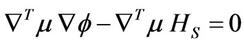 (1)
(1)
The field intensity due to the current in the winding and the permanent magnet may always be calculated directly by the Biot-Savart law and the magnetic dipole moment per unit volume, respectively. This equation, like the Poisson's equation for electrostatic fields can be solved using finite element method. Maxwell 3D V11.1 a FEM solver for magnetic field was used to calculate the scalar potential  and the magnetic field intensity
 .
.
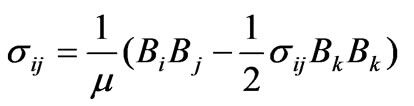
A non uniform distributed force per unit area at the interface between two materials is calculated by use of the Maxwell stress tensor. Since the strain imposed on the material due to magnetostriction is small enough to neglect changes in the density, it can be assumed that the change of permeability is negligible. Thus in tensor notation we have:
 (2)
(2)
where is the Maxwell stress tensor.
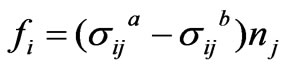
  is the magnetic flux density which is obtained by the multiplication of permeability to the magnetic flux density. From the expression given by Woodson and Melcher [12] for an interface between two materials a and b, the traction
 , is given by:
 (3)
(3)
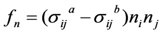
The normal and the tangential traction can be decomposed as follows:
 (4)
(4)
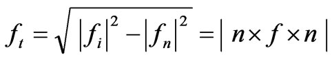 (5)
(5)
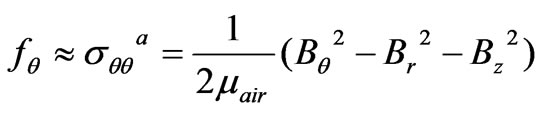
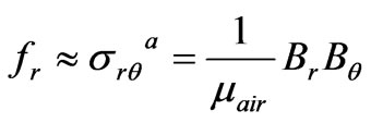
Since , the magnetic traction can be simplified with the introduction of the cylindrical coordinate on the rotor. Along the air gap, the normal and the tangential traction for tooth face are as follows:
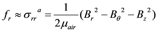 (6)
(6)
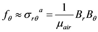 (7)
(7)
But for tooth side which is perpendicular to the air gap the normal and the tangential traction have the following form:
 (8)
(8)
 (9)
(9)
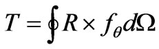
The torque produced for one position can easily be derived from the integration of the shear force along the small air gap with the fact the field distribution inside a closed surface in air remain unchanged if the external sources are removed and replaced by currents and poles on the surface:
 (10)
(10)
3. Modeling
The finite element method has a solid theoretical foundation. It is based on mathematical theorems that guarantee an asymptotic increase of the accuracy of the field calculation towards the exact solution as the size of the finite elements used in the solution process decreases. For time domain solutions the spatial discretization of the problem must be refined in a manner coordinated with the time steps of the calculation according to estimated time constants of the solution (such as magnetic diffusion time constant). Maxwell 3D V11.1 solves the electromagnetic field problems by solving Maxwell’s equations in a finite region of space with appropriate boundary conditions and-when necessary-with user-specified initial conditions in order to obtain a solution with guaranteed uniqueness. In order to obtain the set of algebraic equations to be solved, the geometry of the problem is discretized automatically into tetrahedral elements. All the model solids are meshed automatically by the mesher. The assembly of all tetrahedra is referred to as the finite element mesh of the model or simply the mesh. Inside each tetrahedron, the unknowns characteristic for the field being calculated are represented as polynomials of second order. Thus, in regions with rapid spatial field variation, the mesh density needs to be increased for good solution accuracy (see also adaptive mesh refinement).
Solving an electromagnetic field problem is always based on solving Maxwell’s equations. However the process of obtaining the solution is typically based on solving a second order consequence of Maxwell’s equations with the consideration of applicable constitutive equations. At the same time-as a rule-a subset of complete Maxwell’s equations is considered according to characteristic aspects of the application. Thus for reasons of efficiency of the solution, applications are classified as electrostatic, magnetostatic, frequency domain or time domain and as a consequence a specific type of solver is used in each case. This allows the users to obtain the solution with the desired accuracy but always within the limits of the fundamental assumptions made when the application was classified along the lines of the above mentioned criteria. The guide lines that can be used to correctly identify the type of solution to use are mentioned in the following paragraphs. The unknowns for each type of solution can be different, depending on the formulation.
The solution process for 3D transient applications poses several challenges not apparent for other solver types. For instance, the behavior of fields is more complex than it is for static or steady-state applications, and a special finite element mesh structure is required in order for the software to accurately represent the physics. For 3D transient applications, the behavior of the fields is more complex than it is for static or steady-state applications. A diffusion of the magnetic field into the materials occurs in 3D transient situations. The distribution of the magnetic field inside objects typically has a number of spatial harmonics, which usually means the time step used in the analysis should be less 7 (sometimes much less) than the magnetic diffusion time constant. These time constants depend upon the geometry of objects and also upon their respective material properties. Since eddy currents are usually considered in conductive objects, a special finite element mesh structure is required in order to accurately capture the physics. In general, a careful planning of the (manual) meshing process is required in order to achieve an accurate solution with the available hardware resources. The three dimensional view of the Brushless DC motor is shown in Figure 1.
4. Simulation Results
It is assumed that the square voltages with amplitude of 311 V and frequency of 60 Hz are applied to the brushless DC motor as shown in Figure 2. The brushless DC motor is simulated in the interval of 0 to 0.02 seconds with 0.002s of time step. The magnitude of flux density in times of 0.004s, 0.006s, 0.008s, 0.01s, 0.012s, 0.014s, 0.016s, 0.018s and 0.02s are shown in Figures 3-11. Also, the diagrams of the torque and the force in the z, y and x directions are shown in Figures 12-17 respectively.
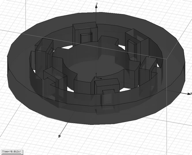
Figure 1. Three dimensional brushless DC motor
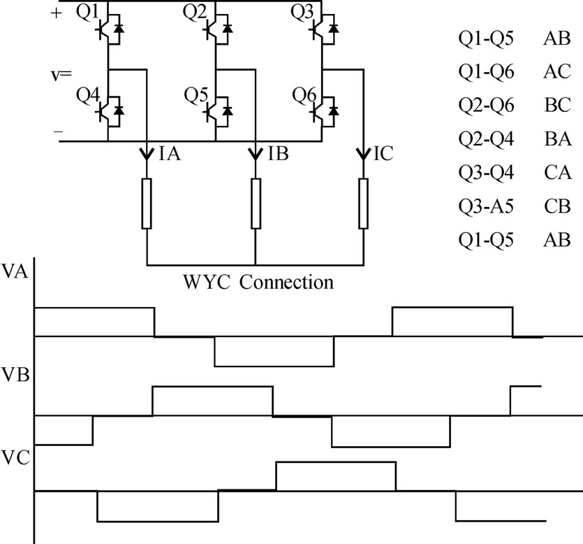
Figure 2. Input voltage waveforms and stator excitation inverter
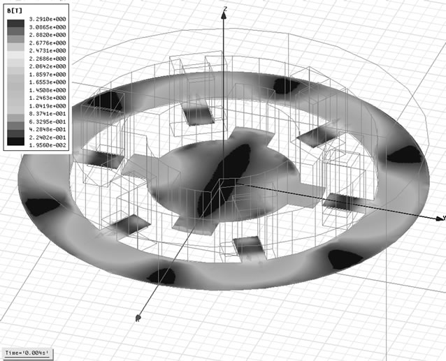
Figure 3. Magnetic flux density in 0.004 s
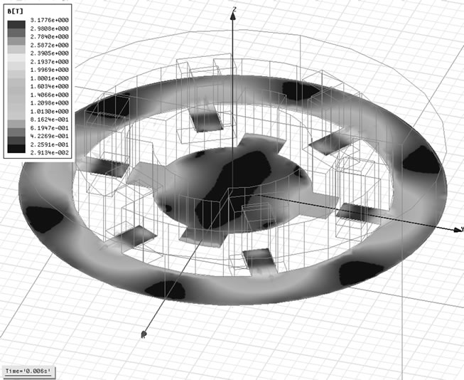
Figure 4. Magnetic flux density in 0.006 s
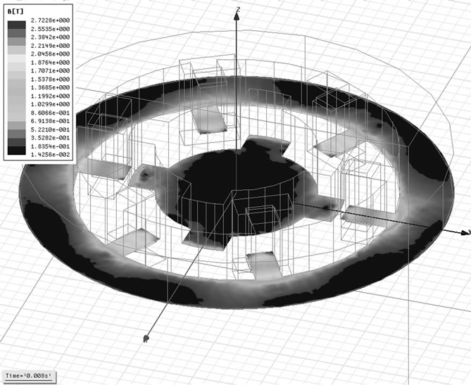
Figure 5. Magnetic flux density in 0.008 s
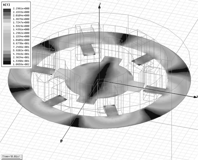
Figure 6. Magnetic flux density in 0.01 s
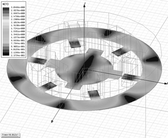
Figure 7. Magnetic flux density in 0.012 s
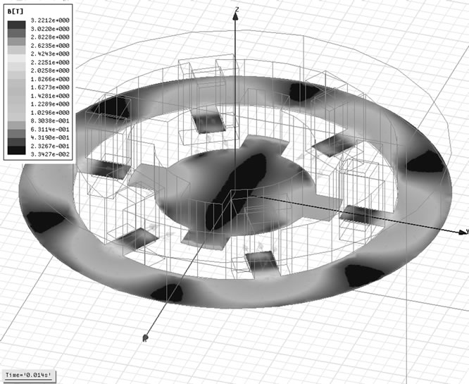
Figure 8. Magnetic flux density in 0.014 s
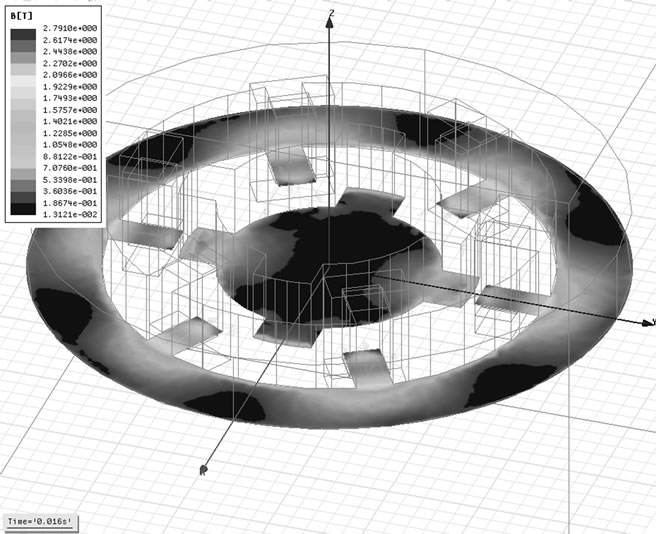
Figure 9. Magnetic flux density in 0.016 s
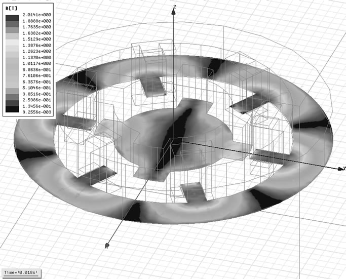
Figure 10. Magnetic flux density in 0.018 s
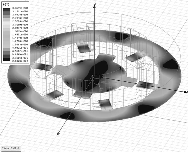
Figure 11. Magnetic flux density in 0.02 s
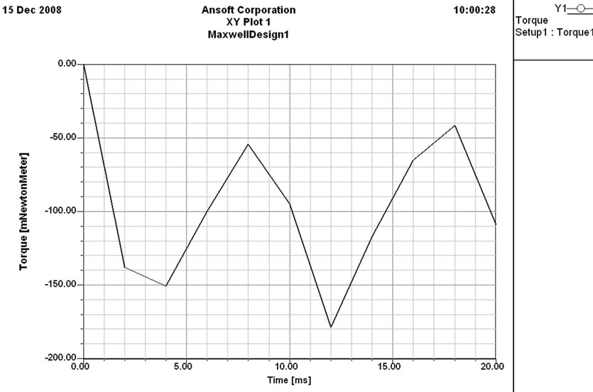
Figure 12. Torque in z-direction
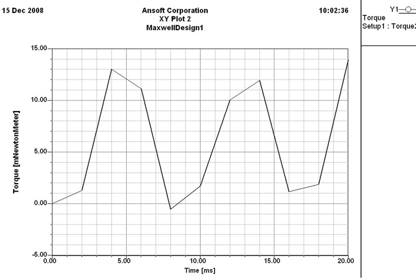
Figure 13. Torque in y-direction
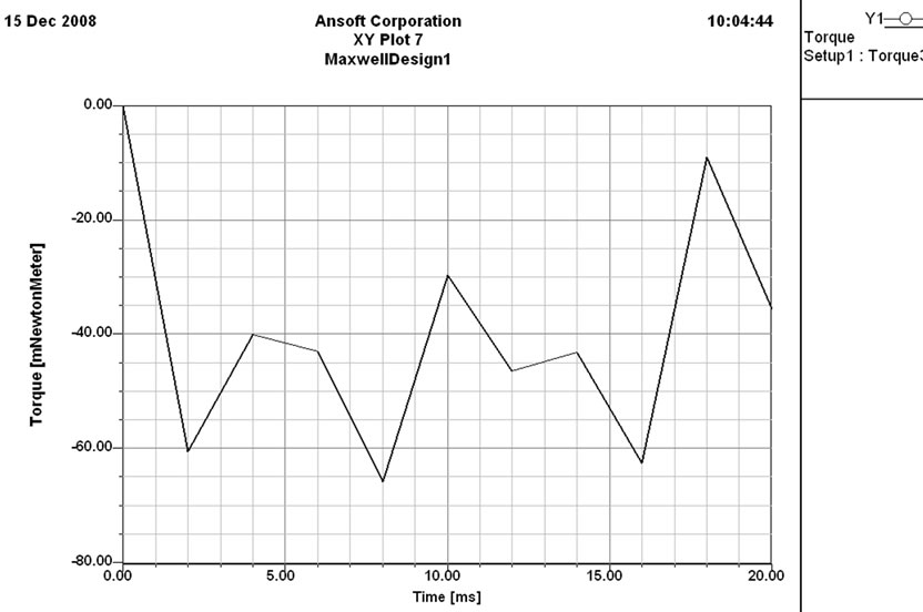
Figure 14. Torque in x-direction
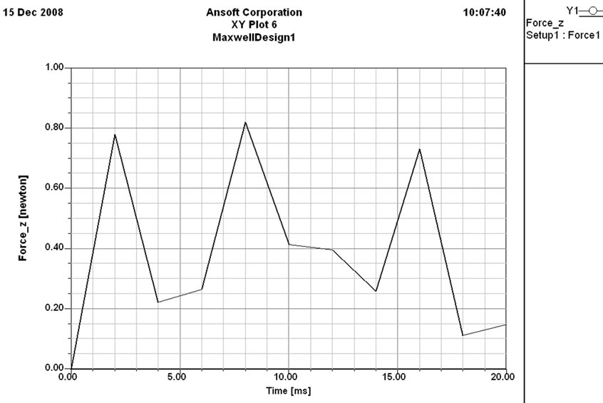
Figure 15. Force in z-direction
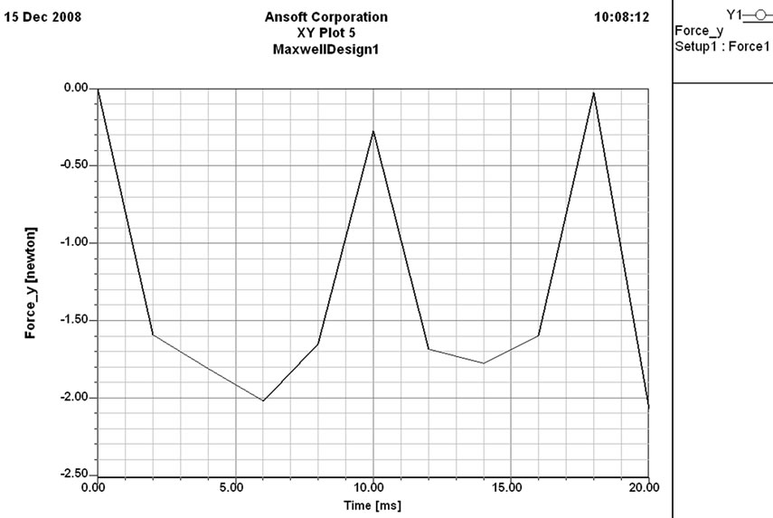
Figure 16. Force in y-direction
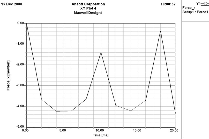
Figure 17. Force in x-direction
5. Conclusions
A method for the analysis of the magnetic force and the torque in a brushless DC motor has been presented from the finite element method and Maxwell stress tensor, so that the characteristics of the magnetic force and the torque can be predictable. Shear force existing in a small air gap produces the torque. The permanent magnet and the teeth geometry produces the reluctant torque, which increases the magnetic field of the teeth corner with the direction to move the rotor to the equilibrium position. The commutating torque is produced by the interaction of the permanent magnet and the current which increases the magnetic field concentration of the teeth corner in the moving direction and decreases it in the opposite direction and the simulation software has analyzed nicely the performance of the brushless DC motor in the transient state.
REFERENCES
- M. Marinescu and N. Marinescu, “Numerical computation of torques in permanent magnet motors by Maxwell stresses and energy method,” IEEE Transactions on Magnetics, Vol. 24, No. 1, pp. 463-466, 1988.
- J. Mizia, K. Adamiak, A. R. Eastham, and G. E. Dawson, “Finite element force calculation: Comparison of methods for electric machine,” IEEE Transactions on Magnetics, Vol. 24, No. 1, pp. 447-450, 1988.
- N. Boules, “Prediction of no-load flux density distribution in permanent magnet machines,” IEEE Transactions on Industry Applications, Vol. IA-21, No. 3, pp. 633-643, 1985.
- J. C. Sabonnadiere, A. Foggia, J. F. Imhoff, G. Reyne, and G. Meunier, “Spectral analysis of electromagnetic vibrations in DC machines through the finite element method,” Digests of the 1989 IEEE Intermag Conference, P. Ec-07, 1989.
- Y. Lefevre, B. Davat, and M. Lajoie-Mazenc, “Determination of synchronous motor vibrations due to electromagnetic force harmonics,” IEEE Transactions on Magnetics, Vol. 25, No. 4, pp. 2974-2976, 1989.
- B. S. Rahman and D. K. Lieu, “The origin of permanent magnet induced vibration in electric machines,” ASME Journal of Vibration and Acoustics, Vol. 113, No. 4, pp. 476-481, 1991.
- G. H. Jang and D. K. Lieu, “Vibration reduction in electric machine by magnet interlacing,” IEEE Transactions on Magnetics, Vol. 28, No. 5, pp. 3024-3026, 1992.
- G. H. Jang and D. K. Lieu, “Vibration reduction in electric machine by interlocking of the magnets,” IEEE Transactions on Magnetics, Vol. 29, No. 2, pp. 1423-1426, 1993.
- P. Kurronen, “Torque vibration model of axial-flux surface-mounted permanent magnet synchronous machine,” Dissertation, Acta Universitatis Lappeenrantaensis 154, ISBN 951-764-773-5, pp. 123, 2003.
- P. Salminen, “Fractional slot permanent magnet synchronous motors for low speed applications,” Dissertation, Acta Universitatis Lappeenrantaensis 198, Finland, pp. 150, 2004.
- T. Heikkilä, “Permanent magnet synchronous motor for industrial applications-analysis and design,” Dissertation, Acta Universitatis Lappeenrantaensis 134, ISBN 951-764-699-2, pp. 109, 2002.
- H. Woodson and J. Melcher, “Electromechanical dynamics, Part II: Fields, forces, and motion,” The Robert E. Krieger Publishing Company, New York, pp. 445-447, 1985.