Int'l J. of Communications, Network and System Sciences
Vol.7 No.7(2014), Article
ID:47663,9
pages
DOI:10.4236/ijcns.2014.77022
Unsupervised Neural Network Approach to Frame Analysis of Conventional Buildings
Lácides R. Pinto1, Alejandro R. Zambrano2
1Universidad de La Guajira, UNIGUAJIRA, Riohacha, Colombia
2Universidad Nacional Experimental Politécnica, UNEXPO, Puerto Ordaz, Venezuela
Email: lacidesrafael@yahoo.com, arzambrano@unexpo.edu.ve
Copyright © 2014 by authors and Scientific Research Publishing Inc.
This work is licensed under the Creative Commons Attribution International License (CC BY).
http://creativecommons.org/licenses/by/4.0/


Received 28 May 2014; revised 20 June 2014; accepted 30 June 2014
Abstract
In this paper, an Artificial Neural Network (ANN) model is used for the analysis of any type of conventional building frame under an arbitrary loading in terms of the rotational end moments of its members. This is achieved by training the network. The frame will deform so that all joints will rotate an angle. At the same time, a relative lateral sway will be produced at the rth floor level, assuming that the effects of axial lengths of the bars of the structure are not altered. The issue of choosing an appropriate neural network structure and providing structural parameters to that network for training purposes is addressed by using an unsupervised algorithm. The model’s parameters, as well as the rotational variables, are investigated in order to get the most accurate results. The model is then evaluated by using the iteration method of frame analysis developed by Dr. G. Kani. In general, the new approach delivers better results compared to several commonly used methods of structural analysis.
Keywords: Structural Analysis, Neural Networks, Unsupervised Training, End Moments, Rotational End Moments

1. Introduction
In the past decades, great strides have been taken in developing frame analysis. Throughout the evolution of structural science, most of the work has been done regarding frame analysis. However, the elasticity theory is available for all approaches.
Four approaches have been presented. The strength of materials approach is the simplest one among them. It is suitable for simple structural members which are subjected to a specific loading. For the analysis of entire systems, this approach can be used in conjunction with static. The solutions are based on linear isotropic infinitesimal elasticity and Euler-Bernoulli beam theory. A second approach, called moment distribution method, was commonly used in the 1930’s. Its essential idea involves no mathematical relations other than the simplest arithmetic [1] . In order to understand the achievement of moment distribution approach, it would be helpful reviewing developments of elasticity theory and its fundamental principles, as it applies to statically indeterminate structures. The iteration method of frame analysis developed by G. Kani [2] , has proved to be extremely satisfactory for structure analysis. Nowadays the moment distribution approach is no longer commonly used due to the fact that computers have changed the way in which engineers evaluate structures. A third method is referred to as the matrix approach. Some believe that during the 1920’s or the early 1930’s, somebody working for the Britain or German aircraft industry was the first person ever to write down stiffness [3] . The major steps in the evolution of Matrix Structural Analysis (MSA) are found in the fundamental contributions of four main authors: Collar, Duncan, Argyris and Turner. Between 1934 and 1938 Collar and Duncan [4] published the first papers which introduced the representation and terminology for matrix systems that are used today. In 1930 they formulated discrete aero elasticity in matrix form. The first couple of journal-published papers and the first book in the field appeared in 1934-1938. The second breakthrough in matrix structural analysis emerged among 1954 and 1955, when Professor Argyris systemized a formal unification of Force and Displacement Methods using dual energy theorems [5] . M. Turner proposed in 1959 the Direct Stiffness Method of structural analysis [6] , one that has undergone the most dramatic changes: an efficient and general computer-based implementation of the incipient Finite Element Method (FEM). Nowadays it can find other models like the Finite Volume Model [7] , used to solve fluids dynamics problems.
Recently, the neural network approach had been applied to many branches of science. This approach is becoming a strong tool for providing structural engineers with sufficient details for design purposes and management practices.
This paper evaluates a neural network approach on frame analysis using an unsupervised algorithm. The results are obtained programming the entire formulation of the algorithm using MATLAB. The aim of the study is to estimate the rotational end moment, and this is depicted in Figure 1.
2. Artificial Neural Networks
An ANN is an information processing system which operates on inputs to extract information, and produces outputs corresponding to the extracted information [8] . Also called connectionists models, parallel distributed processing models and neuromorphic systems, its structure was modeled after that of the human brain and its components. There exist a variety of ANN models and learning procedures. Feed forward networks are well known approaches for prediction [9] -[11] and database processing applications. In this type of ANN, the weighted and biased links feed activation functions from the input layer to the output layer in forward direction. Learning in neural networks comprises adjusting the weights and biases of links. It can be found in the literature [12] -[16] that neural networks had been successfully applied to solve structural problems like damage identification and optimum design of structures, but only taking into account supervised training, which means the necessity of a training set including the patterns and targets. In this paper, we propose a novel ANN architecture with an unsupervised training to solve a structural problem. The success of applying such self-supervised neural networks to any problem depends on training the neural network with sufficient range of input data and adequate operating conditions.
3. General Architecture of Proposed Network
An artificial neural network model is a system composed of many simple processors, each having a local memory. Processing elements are connected by unidirectional links that carry discriminating data. The linear feed forward net has been found to be a suitable one for training techniques. Outputs of neurons in one layer are transferred to their corresponding neuron in another layer through a link that amplifies or inhibits such outputs through weighting factors. Except for the processing elements of the input layer, the input of each neuron is the sum of the weighted outputs of the node in the prior layer and a bias. Each neuron is activated according to its input, activation function, and threshold value.
Figure 2 shows the general feed-forward multilayer network model, including two hidden layers. The distribution factors beams of the input layer constitutes the neurons inputs in layer (L1), representing a set of variables
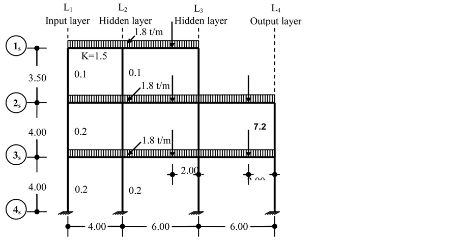
Figure 1. Building frame under any given loading.
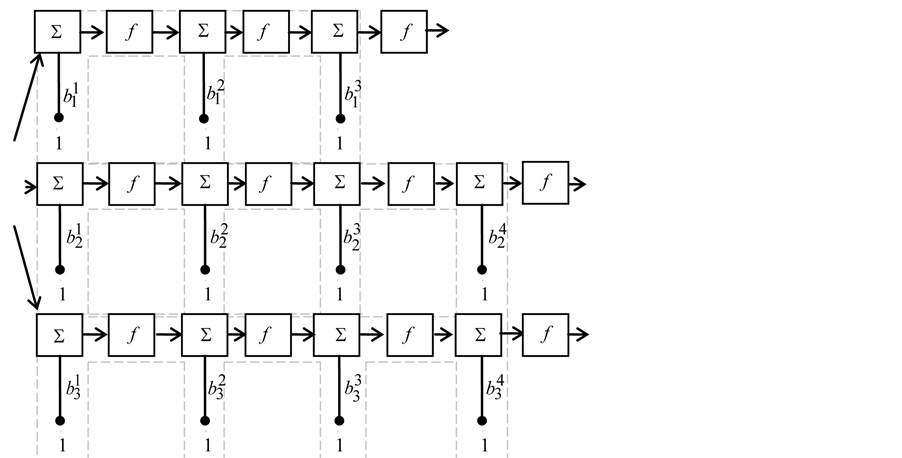
Figure 2. Feed-forward multilayer network.
(x1, x2, x3)T.
The inputs and outputs for the ith neuron are:
 (1)
(1)
 (2)
(2)
where fi constitutes an activation function (linear transfer function). Its behavior is that of a threshold function, in which the output of the neuron is generated if a threshold level, is reached. The net input and output to the jth neuron are similarly treated as in (1) and (2).
Figure 3 shows a neuron simulating a typical processing element in the neural network. The neuron performs a sum-of-products calculation using the input and the connections weights, adding then the threshold value from
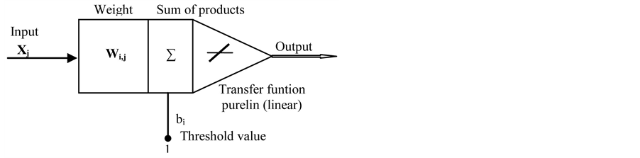
Figure 3. Output processing in a network.
each neuron of the layer, and passing this argument to the transfer function to compute the output. The net input and outputs to and from the ith neuron of the Lth layer are:
 (3)
(3)
And the error,
 (4)
(4)
The output for the  neuron in the
 ![]() layer at the
layer at the  iteration is:
 (5)
(5)
The output for the  neuron in the
 ![]() layer at the
layer at the  iteration is:
 (6)
(6)
Specifically,  is represented by a linear transfer function:
 (7)
(7)
But  represents the input xj for the ith neuron and
  represents its weight, such that,
 , and
, and .
.
Consequently,
 (8)
(8)
where  represents the output variation for two consecutive iterations, and
  acts as a threshold value.
4. Network Algorithm
The connectivity of the neural network model allows processors on one level to communicate with each neuron at the next level. Each processing element in one layer is connected to its corresponding processing element in the next one by the means of an excitatory weight and bias. This is known as a “locally-connected” topology. Discrepancies between actual and target output values results in evaluation of weights and bias changes. After a complete presentation of the training data, a new set of weights and biases are obtained, and new outputs are again evaluated in a feed-forward manner until a specific tolerance for error is obtained. Unsupervised training uses unlabeled training data and requires no external teaching.
In our neural network model, a processing element’s input is connected to a specific node. The node has associated node function which carries out local computation based on the input and bias values. In the input layer, the value of Wij represents the synaptic weight between the recipient node, whose activity is xi, and the previous node whose activity is xj.
There are four descriptors used in the algorithm definition:
• Equation type: Algebraic, the net performs calculations determined primarily by the state of the network.
• Connection topology: The connectivity of the network is the measure of how many processors on one level communicate with each processor at the next level. This is the “locally-connected” topology we discussed earlier, and for a one-dimensional space the matrix will be banded diagonally.
• Processing scheme: Nodes in the network are updated synchronously, since the network output at the current iteration depends entirely on its prior state.
• Synaptic transmission mode: The neural network model takes neural values multiplied by synaptic weights summed across the input to a neuron. The neuron acts on the summed value and its output is multiplied by weights and used as an input for other neurons.
It is known that supervised learning in neural networks based on the popular back propagation method can be often trapped in a local minimum of the error function. How did the proposed algorithm with the “locally-connected” topology overcome such question? This will be asked in a future paper, as well as the characteristics and properties, in detail, of the proposed model. The complexity of the model in the case we have more than two hidden layers depends on the structure to be analyzed: one neuron corresponds to one node in the structure, and the unsupervised training algorithm can deal with any building frame, that means, with any neurons configuration.
5. Selecting Structural Analysis Parameters
The most pertinent variables in structural analysis are the  and
and  fixed end moments induced at the ends of the members under the action of the external loads. Assuming the ends to be completely fixed,
 is termed as the rotational end moment due to rotation
  (expressed in radians) for the
end;  is similarly termed as the rotational end moment due to rotation
  (also expressed in radians) for the
  end.
end.  is the displacement moment in the column consisting of the lateral displacement due to the floor sway,
  is the same for all the members meeting at the
  node, while
 is a distribution factor for the
  member, and
  is the lateral displacement distribution factor.
  represents the stiffness for the
  and
and , the sum of stiffness for all the members meeting at the node
 ![]() These parameters are presented in dimensionless form in several previous studies. Table 1 shows a summary of the most effective dimensionless parameters, which are commonly used for investigating the structural analysis problem.
These parameters are presented in dimensionless form in several previous studies. Table 1 shows a summary of the most effective dimensionless parameters, which are commonly used for investigating the structural analysis problem.
The final expression developed for the total end moments  is, for beams:
 (9)
(9)
And for columns:
 (10)
(10)
In the frame analysis developed in the neural network model, the final end moments  and
and  are determined by finding out the different components
 ,
,  and
and  separately, and then adding them up as per equations (9) and (10). The components of final end moments will be considered positive in clockwise.
6. Training the Network
The distribution factors corresponding to the first layer of the frame’s nodes are presented as an input vector to the input layer, and rotational end moments  and
and , as the outputs. In other words, the input layer contains three neurons, while the output layer contains five. Between the two layers, there are hidden layers that

Table 1 . Structural analysis parameters.
contain a suitable number of neurons. The network was trained with seven iterations. The number of neurons in the hidden layers and adjustable parameters like weights and biases were determined by the number of nodes in the frame, the distribution factors and the rotational end moments.
For any member ,
,  is expressed in terms of the fixed end moments
  and the far end rotational moments
 , as follows:
 (11)
(11)
The values  are then found by adding up the fixed end moments acting at an
  node.
node.
7. The Procedure
The procedure depends on the solution of three problems for the determination of member constants on fixed end moments, the stiffness at each end of member, and of the over-carry factor (distribution factors  for the rotational end moments and distribution factors
 ![]() for the lateral displacement moments) at each end for each member of the frame under consideration. The determination of these values is not a part of the presented approach.
for the lateral displacement moments) at each end for each member of the frame under consideration. The determination of these values is not a part of the presented approach.
The network has four layers, three inputs and five output values. The function network creates the net, which generates the first layer weights and biases for the four linear layers required for this problem. These weights and biases can now be trained incrementally using the algorithm. The network must be trained in order to obtain first layer weights and biases. For the second, third and fourth layers, the weights and biases are modified in response to network’s inputs and will lead to the correct output vector. There are not target outputs available. The linear network was able to adapt very quickly to the change in the outputs. The fact that it takes only seven iterations for the network to learn the input pattern is quite an impressive accomplishment.
The scheme for entering the calculations systematically is shown in Figure 2. The procedure explained above, is best illustrated by solving the structure shown in Figure 1, which is loaded in a rather complex fashion. The distribution factors for nodes 1, 2 and 3 constitute the net’s input vector.
The fixed end moments for the different loaded members are calculated by using the standard formula available in any structural handbook. Having completed these preliminary calculations, the training can be initiated. The network was set up with the three parameters (distribution factors of the beam) as the input, and the rotational end moments due to rotation as the outputs determined by the first layer.
The calculation starts in the input layer and continues from one layer to the next. Such calculation is carried out quickly. After 6 or 7 iterations have been performed, as explained earlier, it will be noted that there is little or no change in the values of two consecutive sets of calculations. The calculations are now stopped and the values of the last iteration are taken as the correct ones, with the previous values being ignored. For the sake of clarity, these final values have been indicated separately in Figure 1.
8. Comparison with Kani’s Method
A comparison between the presented ANN model and Kani’s method was performed on the same example, and it can be shown in Figure 4 and Figure 5. A discrepancy ratio  was used for comparison, where
is the rotational end moment (output network) or total end moment and  is Kani’s result. The mean value
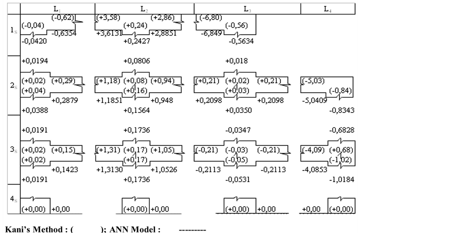
Figure 4. Rotational end moments with lateral displacement.
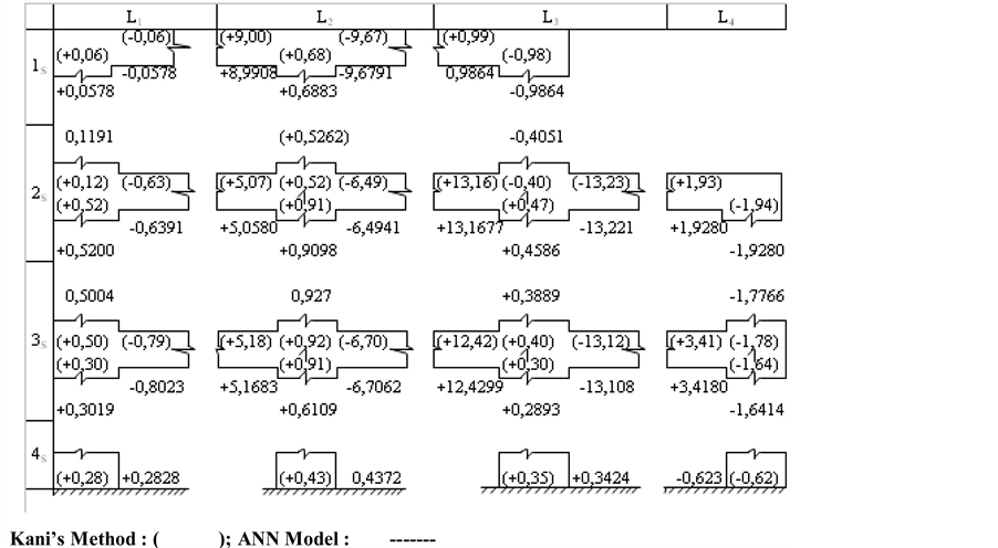
Figure 5. Total end moments with lateral displacement.
 and the standard deviation σ are
  and
and , respectively. The comparison is shown in Table 2 and Table3 From looking at the table, one may conclude that the presented model gives a better agreement with Kani’s method. A group of 15 nodes was used for verification. Figure 4 and Figure 5 shows the nodes of the structure under study, and also the members who access the aforementioned nodes. In these figures we present the comparison of some of the results: rotational moments at the extremes of members obtained with the application of G. Kani Method (distribution moments: these are the values shown in parentheses), and the results of the rotational moments calculated at the ends on the bars of the structure through the
Table 2 . Accuracy of formulas for rotational end moments.
Table 3. Accuracy of formulas for total end moments.
analysis executed by neural topology (whose values are outside the parentheses) that can improve the accuracy and speed of the results.
9. Conclusions
Artificial neural networks are parallel computational models since the computation of the components ,
, and
and  can be used with advantage to extend ANN model to the solution of complex problems. The idea can be used also in the solution of continuous beams on elastic supports, as well as for frames with inclined legs and Vierendeel girders. A very important feature of these networks is their adaptive nature where “learning by example” replaces “programming or making functions” in solving problems. The ANN model ought to be preferred over the Kani’s method, because:
1) The networks, as fine-grained parallel implementations of linear systems, can overcome other approaches.
2) ANNs are very fast even on regular PCs. Enormous data sets can be processed, in comparison with traditional approaches.
3) The presented ANN model is constructed by using only structural model, and it has no boundary conditions in application.
4) Site engineers can calculate rotational moments ,
,  and displacement moments
  using the ANN without prior knowledge of the structural analysis theories, providing them with the knowledge of the bounds of the parameters used to generate the ANN.
5) Artificial neural network models can accept any number of effective variables as input parameters without omission or simplification, as commonly done in conventional approaches.
Acknowledgements
L. R. P. M. thanks to Prof. Alfonzo G. Cerezo for his advice developing this work.
References
- Cross, H. (1949) Analysis of Continuous Frames by Distributing Fixed-End Moments. Numerical Methods of Analysis in Engineering. Successive Corrections. Grinter, L.B., Ed., Macmillan, New York.
- Kani, G. (1957) Die Berechnung Mehrstockinger, Rahmen, Konrad Wittwer Verlag. Verlag Konrad Wittwer, Stuttgart.
- Felippa, C.A. (1995) Parametrized Unification of Matrix Structural Analysis: Classical Formulation and D-Connected Elements. Finite Elements in Analysis and Design, 21, 45-74.
http://dx.doi.org/10.1016/0168-874X(95)00027-8 - Duncan, W.J. and Collar, A.R. (1934) A Method for the Solution of Oscillations Problems by Matrices. Philosophical Magazine Series 7, 17, 865.
- Argyris, J.H. and Kelsey, S. (1960) Energy Theorems and Structural Analysis. Butterworths, London. http://dx.doi.org/10.1007/978-1-4899-5850-1
- Turner. M.J. (1959) The Direct Stiffness Method of Structural Analysis. Structural and Materials Panel Paper, AGARD Meeting, Aachen.
- Eymard, R., Gallouet, T. and Herbin, R. (2000) Handbook for Numerical Analysis. Ciarlet, P.G., Lions, J.L., et al., Eds., North Holland, Amsterdam, 715-1022.
- Freeman, J.A. and Skapura, D.M. (1992) Neural Networks Algorithms, Applications, and Programming Techniques. Addison-Wesley Publishing Company, Inc., Boston.
- Karunanithi, N., Grenney, W.J., Whitly, D. and Bovee, K. (1994) Neural Network for River Flow Prediction. Journal of Computing in Civil Engineering, 215-220.
- Nagy, H., Watanabe, K. and Hirano, M. (2002) Prediction of Sediment Load Concentration in Rivers Using Artificial Neural Network Model. Journal of Hydraulic Engineering, 128, 588-595.
http://dx.doi.org/10.1061/(ASCE)0733-9429(2002)128:6(588) - AFCA International (1988) DARPA Neural Network Study. Library of Congress Cataloging, USA, 131-133.
- Gupta, T. and Sharma, R.K. (2011) Structural Analysis and Design of Buildings Using Neural Network: A Review. International Journal of Engineering and Management Sciences, 2, 216-220.
- Chandwani, V., Agrawal, V. and Nagar, R. (2013) Applications of Soft Computing in Civil Engineering: A Review. International Journal of Computer Applications, 81, 13-20.
- Arangio, S. (2013) Neural Network-Based Techniques for Damage Identification of Bridges: A Review of Recent Advances. Civil and Structural Engineering Computational Methods, Chapter 3. Saxe-Coburg Publications, Stirlingshire, 37-60.
- Sirca Jr., G.F. and Adeli, H. (2012) System Identification in Structural Engineering. Scientia Iranica, 19, 1355-1364. http://dx.doi.org/10.1016/j.scient.2012.09.002
- Salajegheh, E. and Gholizadeh, S. (2005) Optimum Design of Structures by an Improved Genetic Algorithm Using Neural Networks. Advances in Engineering Software, 36, 757-767.
http://dx.doi.org/10.1016/j.advengsoft.2005.03.022