Journal of Intelligent Learning Systems and Applications
Vol.08 No.03(2016), Article ID:69446,12 pages
10.4236/jilsa.2016.83005
Lymph Diseases Prediction Using Random Forest and Particle Swarm Optimization
Waheeda Almayyan
Department of Computer Science and Information Systems, College of Business Studies, Public Authority for Applied Education and Training, Kuwait City, Kuwait

Copyright © 2016 by author and Scientific Research Publishing Inc.
This work is licensed under the Creative Commons Attribution International License (CC BY).
http://creativecommons.org/licenses/by/4.0/


Received 3 May 2016; accepted 30 July 2016; published 3 August 2016
ABSTRACT
This research aims to develop a model to enhance lymphatic diseases diagnosis by the use of random forest ensemble machine-learning method trained with a simple sampling scheme. This study has been carried out in two major phases: feature selection and classification. In the first stage, a number of discriminative features out of 18 were selected using PSO and several feature selection techniques to reduce the features dimension. In the second stage, we applied the random forest ensemble classification scheme to diagnose lymphatic diseases. While making experiments with the selected features, we used original and resampled distributions of the dataset to train random forest classifier. Experimental results demonstrate that the proposed method achieves a remarkable improvement in classification accuracy rate.
Keywords:
Classification, Random Forest Ensemble, PSO, Simple Random Sampling, Information Gain Ratio, Symmetrical Uncertainty

1. Introduction
Nowadays, Computer-Aided Diagnosis (CAD) applications have become one of the key research topics in medical biometrics diagnostic tasks. Medical diagnosis depends upon the experience of the physician beside the existing data. Consequently, a number of articles suggested several strategies to process the physician’s analysis and judgment tasks about actual clinical assessments [1] . With reasonable success, machine-learning techniques have been applied in constructing the CAD applications due to its strong capability of extracting complex relationships in the medical data [2] .
Raw medical data requires some effective classification techniques to support the computer-based analysis of such voluminous and heterogeneous data. Accuracy of clinically diagnosed cases is particularly important issue to be considered during classification. In most cases the size of medical datasets is usually great, which directly affects the complexity of the data mining procedure [3] . So, the large-scale medical data is considered a source of significant challenges in data mining applications, which involves extracting the most descriptive or discriminative features. Thus, feature reduction has a significant role in eliminating irrelevant features from medical datasets [4] [5] . Dimensionality reduction procedure aims to reduce computational complexity with the possible advantages of enhancing the overall classification performance. It includes eliminating insignificant features before model implementation, which makes screening tests faster, more practical and less costly and this is an important requirement in medical applications [6] .
The lymphatic system is a vital part of the immune system in removing the interstitial fluid from tissues. It absorbs and transports fats and fat-soluble vitamins from the digestive system and delivers these nutrients to the cells of the body. It transports white blood cells to and from the lymph nodes into the bones. Moreover, it transports antigen-presenting cells to the lymph nodes where an immune response is stimulated.
Different medical imaging techniques have been used for the investigation of the lymphatic channels and lymph glands status [7] . The current state of lymph nodes with obtained data from lymphography technique can ascertain the classification of the investigated diagnosis [8] . The enlargement of lymph nodes can be an index to several conditions and extends to more significant conditions that threat life [9] . The study of the lymph nodes is important in diagnosis, prognosis, and treatment of cancer [10] . Therefore, the main contribution of this paper is to investigate the effectiveness of the suggested technique in diagnosing the lymph disease problem.
In this article, a CAD system based on random forest ensemble classifier is introduced to improve the efficiency of the classification accuracy for lymph disease diagnosis. The difference between this article and other articles that address the same topic is that a strong ensemble classifier scheme has been created by combining PSO feature selection and random forest decision tree methods, which yields more efficient results than any of the other methods tested in this paper.
Several approaches have been investigated using conventional and artificial intelligence techniques in order to evaluate the lymphography dataset. Karabulut et al. studied the effect of feature selection methods with NaïveBayes, Multilayer Perceptron (MLP), and J48 decision tree classifiers with fifteen real datasets including lymph disease dataset [11] . The best accuracy was 84.46% achieved using Chi-square FS and MLP. Derrac et al. proposed an evolutionary algorithm for data reduction enhanced by Rough set based feature selection. The best accuracy recorded was 82.65% with 5 neighbors [12] . Madden [13] proposed a comparative study between Naïve Bayes, Tree Augmented Naïve Bayes (TAN) and General Bayesian network (GBN) classifier, with K2 search and GBN with hill-climbing search in which they scored an accuracy of 82.16%, 81.07%, 77.46% and 75.06% respectively. De Falco [14] proposed a differential evolution technique to classify eight databases from the medical domain. The suggested technique scored an accuracy of 85.14% compared to 80.18% using Part classifier. Abellán and Masegosa designed Bagging credal decision trees using imprecise probabilities and uncertainty measures. The proposed decision tree model without pruning scored an accuracy of 79.69% and 77.51% with pruning [15] .
In this article, a two-stage algorithm is investigated to enhance classification of lymph disease diagnosis. In the first stage, a number of discriminative features out of 18 were selected using PSO and several feature selection to reduce the dimension. In the second stage, we used a random forest ensemble classification scheme to diagnose lymphography types. While making experiments with the selected features, we used original and resampled distributions of the dataset to train random forest algorithm. We noticed a promising improvement in classification performance of the algorithm with resampling strategy.
The article commences with the suggested feature selection techniques and the random forest ensemble classifier. Section 4 briefly introduces simple random sampling strategy. Section 5 focuses on the applied performance measures. Section 6 describes the experiment steps and the involved dataset and shows the result of the experiments. The article concludes with conclusion and further research.
2. Feature Selection
The main objectives of the proposed approach are to improve the performance of classification accuracy and obtain the most important features. Essentially, the feature space is searched to reduce the feature space and prepare the conditions for the classification step. This task is carried out using different state-of-the-art dimension reduction techniques, namely Particle Swarm Optimization, Information Gain Ratio attribute evaluation and Symmetric Uncertainty correlation-based measure.
2.1. Particle Swarm Optimization for Feature Selection
The particle swarm optimization (PSO) technique is a population-based stochastic optimization technique first introduced in 1995 by Kennedy and Eberhart [16] . In PSO, a possible candidate solution is encoded as a finite-length string called a particle pi in the search space. All of the particles make use of its own memory and knowledge gained by the swarm as a whole to find the best solution. With the purpose of discovering the optimal solution, each particle adjusts its searching direction according to two features, its own best previous experience (pbest) and the best experience of its companions flying experience (gbest). Each particle is moving around the n-dimensional search space S with objective function . Each particle has a position
  (t represents the iteration counter), a fitness function
  and “flies” through the problem space with a velocity
 . A new position
  is called better than
  iff
iff  [17] .
Particles evolve simultaneously based on knowledge shared with neighbouring particles; they make use of their own memory and knowledge gained by the swarm as a whole to find the best solution. The best search space position particle i has visited until iteration t is its previous experience pbest. To each particle, a subset of all particles is assigned as its neighbourhood. The best previous experience of all neighbours of particle i is called gbest. Each particle additionally keeps a fraction of its old velocity. The particle updates its velocity and position with the following equation in continuous PSO [17] :
 (1)
(1)
 (2)
(2)
The first part in Equation (1) represents the previous flying velocity of the particle. While the second part represents the “cognition” part, which is the private thinking of the particle itself, where C1 is the individual factor. The third part of the equation is the “social” part, which represents the collaboration amongst the particles, where C2 is the societal factor. The acceleration coefficients (C1) and (C2) are constants represent the weighting of the stochastic acceleration terms that pull each particle toward the pbest and gbest positions. Particles’ velocities are restricted to a maximum velocity, Vmax. If Vmax is too small, particles in this case could become trapped in local optima. In contrast, if Vmax is too high particles might fly past fine solutions. According to Equation (1), the particle’s new velocity is calculated according to its previous velocity and the distances of its current position from its own best experience and the group’s best experience. Afterwards, the particle flies toward a new position according to Equation (2). The performance of each particle is measured according to a pre-de- fined fitness function (Figure 1).
2.2. Information Gain Ratio Attribute Evaluation
Information Gain Ratio attribute evaluation (IGR) measure was generally developed by Quinlan (Quinlan, 1993) within the C4.5 algorithm and based on the Shannon entropy to select the test attribute at each node of the decision tree [18] . It represents how precisely the attributes predict the classes of the test dataset in order to use the “best” attribute as the root of the decision tree.
The expected IGR needed to classify a given sample s from a set of data samples C  is calculated as follow
 (3)
(3)


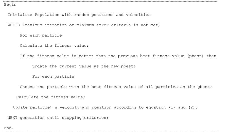
Figure 1. Pseudocode of PSO-based feature selection approach.


where , Ci and |Ci| are the frequency of the sample s in C, the ith class of C and the number of samples in Ci, respectively.
2.3. Symmetrical Uncertainty
Symmetric uncertainty correlation-based measure (SU) can be used to evaluate the goodness of features by calculating between feature and the target class (Fayyad & Irani, 1993; Liu et al., 2002) [19] [20] . The features having greater SU value get higher importance. SU is defined as
 (4)
(4)

where H(X), H(Y), H(X|Y), IG are the entropy of a of X, entropy of a of Y and the entropy of a of posterior probability X given Y and information gain, respectively.
3. Random Forest Ensemble Classification Algorithm
Ensemble learning methods which utilizes ensembles of classifiers such as neural networks ensembles, random forest, bagging and boosting have received an increasing interest because of their ability to deliver an accurate prediction and robust to noise and outliners than single classifiers [21] [22] . The basic idea behind ensembled classifiers is based upon the premise that a group of classifiers can perform better than an individual classifier. In 2001, Breiman proposed a new and promising tree-based ensemble classifier based on a combination tree of predictors such that each tree depends on the values of a random vector sampled independently and with the same distribution for all trees and called it random forest. Random forest classifier consists of a combination of individual base classifiers where each tree is generated using a random vector sampled independently from the classification input vector to enable a much faster construction of trees. For classification, the classification single vote from all trees is combined using a rule based approach (such as, majority voting, product, sum, or Bayesian rule), or based on an iterative error minimization technique by reducing the weights for the correctly classified samples.
In Random Forest, the method to build an ensemble of classifiers can be summarized as follows:
The Random Forest training algorithm starts with constructing multiple trees. In the literature, several methods were used such as random trees, CART, J48, C4.5, etc. In this article we are using the random trees in building the Random Forest classifier with no pruning, which makes it light, from a computational perspective.
The next step is preparing the training set for each tree, which is formed by randomly sampling the training dataset using bootstrapping technique with replacement. This step is called the bagging step [23] and the selected samples are called the in-bag samples; the rest are set aside as out-of-bag samples. For each new training set that is generated, approximately one third of the data in the in-bag set is duplicated (sampling with replacement) and used for building the tree. Whereas, the remaining training samples, out-of-bag, are used to test the tree classification performance. Figure 2 illustrates the data sampling procedure. Each tree is constructed using a different bootstrap sample.
Random Forest increases the diversity of the trees by choosing and using a random number of features (in this work four features) to construct the nodes and leafs of a random tree classifier. According to Breiman [21] [23] , this step minimizes the correlation among the features, decreases the sensitivity to noise in the data and, at the same time, increases the accuracy of classification.
Building a random tree begins at the top of the tree with in-bag dataset. The first step involves selecting a feature at the root node and then splitting the training data into subsets for every possible value of the feature. This makes a branch for each possible value of the attribute. Tree design requires choosing a suitable attribute selection measure for splitting and the selection of the root node to maximize dissimilarity between classes. The information gain (IG) of splitting the training dataset (Y) into subsets (Yi) can be defined as:
 (5)
(5)
If the information gain is positive; the node is split else the node will become a leaf node that would provide a decision of the most common target class in the training subset.
The partitioning procedure is repeated recursively at each branch node using the subset that reaches the branch and the remaining attributes continues until all attributes are selected. The highest information gain of the remaining attributes is selected as the next attribute. Eventually the most occurring target class in the training subset that reached that node is assigned as the classification decision.
The procedure is repeated to build all trees.
After building all trees, the out-of-bag dataset is used to test trees as well as the entire forest. The obtained average misclassification error can be used to adjust the weights of the vote of each tree. In this article, the implementation of the random forest classifier gives each tree the same weight.
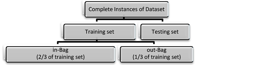
Figure 2. Data partition in constructing random forest trees.
4. Simple Random Sampling
Medical data usually experience class imbalance problems, due to the fact that one class is represented by a considerably larger number of instances than other classes. Subsequently, classification algorithms tend to ignore the minority classes. Simple random sampling has been advised as a good means of increasing the sensitivity of the classifier to the minority class by scaling the class distribution. An empirical study where the authors used twenty datasets from UCI repository has showed quantitatively that classifier accuracy might be increased with a progressive sampling algorithm [24] . Weiss and Provost deployed decision trees to evaluate classification performances with the use of a sampling strategy. Another important study used sampling to scale the class distribution and mainly focus on biomedical datasets [25] . The authors measure the effect of the suggested sampling strategy by the use of nearest neighbor and decision tree classifiers. In Simple random sampling, a sample is randomly selected from the population so that the obtained sample is representative of the population. Therefore, this technique provides an unbiased sample from the original data.
Regarding simple random sampling there are two approaches while making random selection, in the first approach the samples are selected with replacement where the sample can be selected more than once repeatedly with an equal selection chance. In the other approach the selection of samples is done without replacement where the sample can be selected only once, so that each sample in the data set has an equal chance of being selected and once selected it cannot be chosen again [26] .
5. Performance Measures
When the data is inadequate, predicting classification performance of a machine learning method is difficult. Thus, Cross-validation is preferred when the scholar have a small amount of data [27] . When machine-learning methods explore data, decisions must be made on how to split dataset for training and testing. With the intention of estimating the performance of machine learning methods, the lymphography dataset is split into training and testing subsets, afterwards a 10-fold cross-validation, which is a commonly used technique for evaluation, is applied.
The performance of the suggested technique was evaluated by using four commonly used performance metrics, Precision, ROC, MCC and Cohen’s kappa coefficient. The main formulations are defined in Equations (4)-(6), according to the confusion matrix. In the confusion matrix of a two-class problem, TP is the number of true positives that was classified correctly. FN is the number of false negatives that was classified incorrectly. TN is the number of true negatives that was classified as negatives. FP is the number of false positives that was classified as negatives. Accordingly, we can define Precision as:
 (6)
(6)
Receiver Operator Characteristic (ROC) curve is another commonly used measure to evaluate two-class decision problems in Machine Learning. The ROC curve is a standard tool for summarizing classifier performance over a range of tradeoffs between TP and FP error rates [28] . ROC usually takes values between 0.5 for random drawing and 1.0 for perfect classifier performance.
Considering class-imbalanced datasets, such as the case in this database, the Matthews Correlation Coefficient (MCC) is an appropriate measure that considered balanced. It can be used even if the classes are of very different in sizes, as it is a correlation coefficient between the observed and predicted classification decisions. The MCC measure falls within the range of [−1, 1]. The larger the MCC coefficient indicates better classifier prediction. The MCC measure can be calculated directly from the confusion matrix using the following formula:
 (7)
(7)
Additionally, Kappa error or Cohen’s kappa statistics is a recommended measure to compare the performances of different classifiers and hence the quality of selected features. Generally Kappa error value Î [−1,1], so when Kappa error value calculated for classifiers approaches to 1, then the performance of classier is assumed to be more realistic [28] . The Kappa error measure can be calculated using the following formula:
 (8)
(8)
where P(A) is total agreement probability and P(E) is the hypothetical probability of chance agreement.
6. Experimental Study
This lymphography database was first obtained by the University Medical Centre, Institute of Oncology, Ljubljana, Yugoslavia and then it was donated by the same contributors to UCI Machine Learning Repository [29] [30] . It comprised of 148 instances represented by 18 diagnostic features. The classification of the Lymph dataset will be with respect to condition of the subject as normal, metastases, malign lymph or fibrosis. The 18features along with description, mean and standard deviation are listed in Table 1. Each of the classes has the sample sizes of 2, 81, 61 and 4, respectively.
All the experiments were carried in Waikato Environment for Knowledge Analysis (WEKA) a popular suite of data mining algorithms written in Java as follows:
i) RF algorithm ensemble classifier is designed based on 150 trees and 10 random features to build each tree.
ii) The suggested algorithm is trained with lymphographic dataset using 10-fold cross validation strategy to evaluate the classification accuracy on the dataset.
As mentioned earlier, the suggested system for the purpose of enhancement of Lymph diseases diagnosis applied in this study is carried out in two major phases. In the first phase, the feature space is searched to reduce the feature space and prepare the conditions for the next step. This task is carried out using three feature selection techniques, PSO, IGR and SU. For PSO feature selection, population size is 20, number of iterations is 20, individual weight is 0.34 and inertia weight is 0.33. The optimal features of these techniques are summarized in Table 2. It is worth noting that the number of features has remarkably reduced, therefore less storage space is required for the execution of the classification algorithms. This step helped in reducing the size of dataset to only 9 to 13 attributes. Figure 3 visualizes the feature selection techniques agreements. The Venn diagram shows the three feature selection techniques shares the lymphatic, block of afferent, regeneration, early uptake, lymph nodes diminish, changes in lymph, defect in node, changes in node and number of nodes attributes. It also indicates that the early uptake and changes in structure attributes were common between PSO and IGR techniques. Whereas, special forms characteristic was common between IGR and SU techniques.
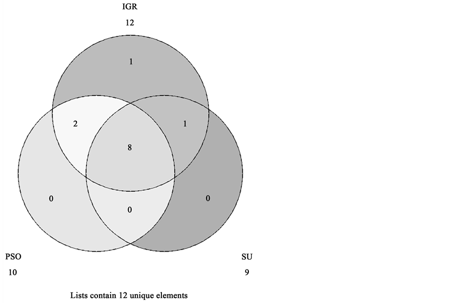
Figure 3. Feature selection techniques agreement.

Table 1. Lymphographic dataset description of attributes.
Table 2. Selected features of lymph disease data set.
Afterwards, the selected features are used as the inputs to the classifiers. For the purpose of classification, three machine-learning classification paradigms, which are considered very robust in solving non-linear problems, are examined to estimate the lymph disease possibility. These methods include C4.5 as decision trees, k-NN as an instance based learner and feed-forward artificial neural network classifier (Multi-layered Perceptron MLP). The k-NN classifier is performed based on Euclidean distance measure for k = 1. While C4.5 classifier was applied with a confidence factor for pruning = 0.25 and a minimum number of instances per leaf of 2. And MLP classifier with a learning rate = 0.3 and momentum = 0.2. In Table 3, we depict the comparative results of the classification performance before and after applying the feature reduction phase that deploy PSO, IGR and SU algorithms to detect the most significant features. As Table 3 is examined, it is seen that before the feature reduction step, the highest precision rate is associated with RF classifier was 84.3% with 18 features. The proposed method based on RF+PSO approach obtained 82.6%, 67.5%, 92.4% and 66.8% for Precision, Recall, MCC, ROC and Kappa, respectively with 10 features. RF+IGR and RF+SU techniques obtained an average
Table 3. Classification performances of lymphographic data―without sampling.
Precision rate of 78.1% and 77.7% with 12 and 9 features, respectively. Clearly we can observe that the PSO helped in reducing the dimension of features. Yet, this step did not improve the classification performance.
Table 4 describes the class distribution, which clearly shows that the lymphography dataset is imbalanced. A common problem with the imbalanced data is that the minority class contributes very little to the standard algorithms accuracy. This unbalanced distribution makes the lymphography dataset suitable to test the effect of simple random sampling strategy. We, therefore, used a simple random sampling approach with replacement to rescale class distribution of the dataset. The class distributions before and after simple random sampling are given in Table 4. The classification performance of this trained algorithm is tested with original distribution, i.e., without resampling, of data using 10-fold cross validation scheme.
Table 5 shows the final classification results after applying the random sampling strategy on the reduced dataset to balance the number of instances in the minority classes. This step contributes to make a more diverse and balanced dataset. As it could be seen from results of Table 5, the highest precision rate before the feature reduction step is associated with k-NN classifier was 92.7% with 18 features. The proposed method based on RF and PSO approach obtained 94%, 89.8%, 98.3% and 92.3% for Precision, MCC, ROC and Kappa error, respectively with 10 features. While the proposed method based on RF and IGR approach obtained 95.4%, 92.5%, 98.4% and 92.3% for Precision, MCC, ROC and Kappa error, respectively with 12 features. In Table 5, it is also seen that the other performance indexes supports this improvement with increasing values compared to un-sampled classification strategy. We can observe that proposed RF+PSO model helped in improving the classification performance with a limited number of features. The results demonstrated that these features are fairly competent to represent the dataset’s class information. In terms of Precision, MCC, ROC and Cohen's kappa coefficient our proposed technique that deploys random sampling technique succeeded in significantly improving the classification accuracy of the minority while the classification accuracy of major class remains high. The outcomes from the suggested technique show better results compared to datasets which are un-sampled and also when these attribute selection techniques are used independently. As can be seen from above results, the proposed method based on RF+PSO has produced very promising results on the classification of the possible lymph diseases patients.
Table 4. Class distribution of the Lymphographic dataset before and after simple random sampling.
Table 5. Classification performance of Lymphographic dataset―with sampling
7. Conclusion
The main goal of medical data mining is to extract hidden information using data mining techniques. One of the positive aspects is to support the analysis of this data. Therefore, accuracy of classification algorithms used in disease diagnosing is certainly an essential issue to be considered. In this article, a random forest classifier approach has been investigated to improve the diagnosis of lymph diseases. The proposed RF + PSO model improved the accuracy performance and achieved promising results. The experiments have shown that the PSO feature selection technique helped in reducing the feature space, whereas adjusting the original data with simple random sampling helped in increasing the region area of the minority class in favor of handling the existing imbalanced data property. The future plan will take into consideration by applying the proposed technique in other medical diagnosis problems.
Acknowledgements
The Public Authority for Applied Education and Training in Kuwait supports this work (grant number BS-14- 02). The author would like to kindly appreciate and gratefully acknowledge, UCI Machine Learning Repository (http://archive.ics.uci.edu/ml/) for obtaining the lymphographic dataset.
Cite this paper
Waheeda Almayyan, (2016) Lymph Diseases Prediction Using Random Forest and Particle Swarm Optimization. Journal of Intelligent Learning Systems and Applications,08,51-62. doi: 10.4236/jilsa.2016.83005
References
- 1. Ciosa, K.J. and Mooree, G.W. (2002) Uniqueness o Medical Data Mining. Artificial Intelligence in Medicine, 26, l-24.
http://dx.doi.org/10.1016/s0933-3657(02)00049-0 - 2. Ceusters, W. (2000) Medical Natural Language Understanding as a Supporting Technology for Data Mining in Healthcare Medical Data Mining and Knowledge Discovery. Cios KJ Editor, Heidelberg: Springer, pp. 32-60,.
- 3. Calle-Alonso, F., Pérez, C.J., Arias-Nicolás, J.P. and Martín, J. (2012) Computer-Aided Diagnosis System: A Bayesian Hybrid Classification Method. Computer Methods and Programs in Biomedicine, 112, 104-113.
http://dx.doi.org/10.1016/j.cmpb.2013.05.029 - 4. Cselényi, Z. (2005) Mapping the Dimensionality Density and Topology of Data: The Growing Adaptive Neural Gas. Computer Methods and Programs in Biomedicine, 78, 141-156.
http://dx.doi.org/10.1016/j.cmpb.2005.02.001 - 5. Huang, S.H., Wulsin, L.R., Li, H. and Guo, J. (2009) Dimensionality Reduction for Knowledge Discovery in Medical Claims Database: Application to Antidepressant Medication Utilization Study. Computer Methods and Programs in Biomedicine, 93, 115-123.
http://dx.doi.org/10.1016/j.cmpb.2008.08.002 - 6. Luukka, P. (2011) Feature Selection Using Fuzzy Entropy Measures with Similarity Classifier. Expert Systems with Applications, 38, 4600-4607.
http://dx.doi.org/10.1016/j.eswa.2010.09.133 - 7. Luciani, A., Itti, E., Rahmouni, A., Michel Meignan, M. and Clement, O. (2006) Lymph Node Imaging: Basic Principles. European Journal of Radiology, 58, 338-344.
http://dx.doi.org/10.1016/j.ejrad.2005.12.038 - 8. Sharma, R., Wendt, J.A., Rasmussen, J.C., Adams, A.E., Marshall, M.V. and Sevick-Muraca, E.M. (2008) New Horizons for Imaging Lymphatic Function. Annals of the New York Academy of Sciences, 1131, 13-36.
http://dx.doi.org/10.1196/annals.1413.002 - 9. Guermazi, A., Brice, P., Hennequin, C. and Sarfati, E. (2003) Lymphography: An Old Technique Retains Its Usefulness. RadioGraphics, 23, 1541-1558.
http://dx.doi.org/10.1148/rg.236035704 - 10. Cancer Research UK.
http://www.cancerresearchuk.org - 11. Karabulut, E.M., Özel, S.A. and Íbrikci, T. (2012) A Comparative Study on the Effect of Feature Selection on Classification Accuracy. Procedia Technology, 1, 323-327.
http://dx.doi.org/10.1016/j.protcy.2012.02.068 - 12. Derrac, J., Cornelis, C., García, S. and Herrera, F. (2012) Enhancing Evolutionary Instance Selection Algorithms by Means of Fuzzy Rough Set Based Feature Selection. Information Sciences, 186, 73-92.
http://dx.doi.org/10.1016/j.ins.2011.09.027 - 13. Madden, M.G. (2009) On the Classification Performance of TAN and General Bayesian Networks. Knowledge-Based Systems, 22, 489-495.
http://dx.doi.org/10.1016/j.knosys.2008.10.006 - 14. De Falco, I. (2013) Differential Evolution for Automatic Rule Extraction from Medical Databases. Applied Soft Computing, 13, 1265-1283.
http://dx.doi.org/10.1016/j.asoc.2012.10.022 - 15. Abellán, J. and Masegosa, A.R. (2012) Bagging Schemes on the Presence of Class Noise in Classification. Expert Systems with Applications, 39, 6827-6837.
http://dx.doi.org/10.1016/j.eswa.2012.01.013 - 16. Kennedy, J. and Eberhart, R.C. (2001) Swarm Intelligence. Morgan Kaufmann Publishers, Burlington.
- 17. Kennedy, J. and Eberhart, R.C. (1997) A Discrete Binary Version of the Particle Swarm Algorithm. Proceedings of the IEEE International Conference on Systems, Man, and Cybernetics, 5, 4104-4108. http://dx.doi.org/10.1109/icsmc.1997.637339
- 18. Quinlan, J.R. (1993) C4.5: Programs for Machine Learning. Morgan Kaufmann Publishers, Burlington.
- 19. Fayyad, U. and Irani, K. (1993) Multi-Interval Discretization of Continuous-Valued Attributes for Classification Learning. Proceedings of the 13th International Joint Conference on Artificial Intelligence, Chambéry, 28 August-3 September 1993, 1022-1027.
- 20. Liu, H., Hussain, F., Tan, C. and Dash, M. (2002) Discretization: An Enabling Technique. Data Mining and Knowledge Discovery, 6, 393-423.
http://dx.doi.org/10.1023/A:1016304305535 - 21. Breiman, L. (2001) Random Forests. Machine Learning, 45, 5-32.
- 22. Dietterich, T.G. (2000) An Experimental Comparison of Three Methods for Constructing Ensembles of Decision Trees: Bagging, Boosting, and Randomization. Machine Learning, 40, 139-157.
http://dx.doi.org/10.1023/A:1007607513941 - 23. Breiman, L. (1996) Bagging Predictors. Machine Learning, 24, 123-140.
- 24. Weiss, G. and Provost, F. (2003) Learning when Training Data Are Costly: The Effect of Class Distribution on Tree Induction. Journal of Artificial Intelligence Research, 19, 315-354.
- 25. Park, B.-H., Ostrouchov, G., Samatova, N.F. and Geist, A. (2004) Reservoir-Based Random Sampling with Replacement from Data Stream. Proceedings of the 2004 SIAM International Conference on Data Mining, 22-24 April 2004, Lake Buena Vista, 492-496.
http://dx.doi.org/10.1137/1.9781611972740.53 - 26. Mitra, S.K. and Pathak, P.K. (1984) The Nature of Simple Random Sampling. The Annals of Statistics, 12, 1536-1542.
http://dx.doi.org/10.1214/aos/1176346810 - 27. Schumacher, M., Hollander, N. and Sauerbrei, W. (1997) Resampling and Cross-Validation Techniques: A Tool to Reduce bias Caused by Model Building? Statistics in Medicine, 16, 2813-2827.
http://dx.doi.org/10.1002/(SICI)1097-0258(19971230)16:24<2813::AID-SIM701>3.0.CO;2-Z - 28. Ben-David, A. (2008) Comparison of Classification Accuracy Using Cohen’s Weighted Kappa. Expert Systems with Applications, 34, 825-832.
http://dx.doi.org/10.1016/j.eswa.2006.10.022 - 29. Cestnik, G., Konenenko, I. and Bratko, I. (1987) Assistant-86: A Knowledge-Elicitation Tool for Sophisticated Users. In: Bratko, I. and Lavrac, N., Eds., Progress in Machine Learning, Sigma Press, Wilmslow, 31-45.
- 30. UCI (2016) Machine Learning Repository.
http://archive.ics.uci.edu/ml/index.html