Journal of Intelligent Learning Systems and Applications
Vol.07 No.03(2015), Article ID:57870,11 pages
10.4236/jilsa.2015.73007
Disparity in Intelligent Classification of Data Sets Due to Dominant Pattern Effect (DPE)
Mahmoud Zaki Iskandarani
Faculty of Science and Information Technology, Al-Zaytoonah University of Jordan, Amman, Jordan
Email: m.iskandarani@hotmail.com
Copyright © 2015 by author and Scientific Research Publishing Inc.
This work is licensed under the Creative Commons Attribution International License (CC BY).
http://creativecommons.org/licenses/by/4.0/


Received 29 April 2015; accepted 7 July 2015; published 10 July 2015
ABSTRACT
A hypothesis of the existence of dominant pattern that may affect the performance of a neural based pattern recognition system and its operation in terms of correct and accurate classification, pruning and optimization is assumed, presented, tested and proved to be correct. Two sets of data subjected to the same ranking process using four main features are used to train a neural network engine separately and jointly. Data transformation and statistical pre-processing are carried out on the datasets before inserting them into the specifically designed multi-layer neural network employing Weight Elimination Algorithm with Back Propagation (WEA-BP). The dynamics of classification and weight elimination process is correlated and used to prove the dominance of one dataset. The presented results proved that one dataset acted aggressively towards the system and displaced the first dataset making its classification almost impossible. Such modulation to the relationships among the selected features of the affected dataset resulted in a mutated pattern and subsequent re-arrangement in the data set ranking of its members.
Keywords:
Pattern Recognition, Neural Networks, Ranking, Datasets, Weight Elimination, Pruning, Mutation, Genetic Algorithms

1. Introduction
The main problem in neural network design and application for many years was the choice of an appropriate network for a given application. In general, network size affects network complexity and learning time, but most importantly it affects the generalization capabilities of the network to accurately predict results for data outside the used training sets. A network with unnecessary complex structure and large connections will definitely fit the training data patterns in the training set but performs very poorly on unknown patterns. On the other hand, a network having a structure simpler than necessary cannot give good results even for patterns included in its training sets.
Emphasis has been given to the development of algorithms that reduce network size by modifying not only the connection weights but also the network structure during training, such as pruning, where unnecessary nodes or connections are eliminated using a sensitivity based measure to indicate how the solution is affected from this change, or modifying the error function of the network in such a way that unnecessary connection weights are pushed gradually to zero during training in a decay like process. Other algorithms start with a small network and gradually build it up by increasing the number of nodes or connections during training. In addition, weight sharing through assigning identical set of weights to each node in a group is also researched and tried. All efforts aimed at improving network design and reducing size and training times without affecting its generalization [1] - [4] .
Network size and connection structure are definitely important in deciding the functionality of the design and the ability to optimize through pruning techniques and algorithms. However, research always approached the used data in terms of its size, validity, selected features, training samples, and cross validation, but hardly touched the issue and possibility that another important factor could lead to over fitting and under fitting of examined data sets and their pattern besides network size, number of connections, training algorithm, cross validation, and pruning.
The hypothesis that a data set processed under the same conditions as the rest of datasets, which will have similar effects on another dataset and the neural algorithm performance in classification and prediction, to the previously mentioned factors in negatively influencing the performance of the designed neural network structure, should be proved and catered for alongside the all-time concerns of neural network designers. If not recognized, this dataset will have devastating effects on the designed neural net, and will disable the network from correct functionality. It will also result in endless trials to modify the design and used algorithms, as the focus will be on traditional variables that lead to such over fit-under fit behavior of the neural system [5] - [7] .
Studying datasets that cause such neural network malfunction is very important as they will reveal specific information which can be traced back to the original process that results in their production. The severe effect of a dataset on the behavior of a well-designed and optimized neural network, when used as a training data set, is worth analyzing [8] [9] .
In this paper, a clear evidence of the existence of the Dominant Pattern (DP) and its undesirable effects in creating chaos and randomness among the rankings of elements in datasets are presented and proved.
2. Methodology
The goal of the proposed approach is to discover the effect of a dominant pattern on the accuracy of classification of neural systems in order to provide better solutions, and to identify hostile datasets that contribute in addition to other factors such as the size, number of layers, number of nodes and interconnections to the failure of the system to converge and correctly classify, which will result in a distorted pattern. Thus, permutations of neural network trials (N), using various parameter settings, until the most promising and well optimized structure is obtained as shown in Figure 1. Instead of training each network separately for each dataset, the same structure is used for all permutations and possible combinations, resulting in identical testing conditions [10] .
Table 1 and Table 2 show the post processed datasets used for training the neural infrastructure in Figure 1.
The four selected features are not apparently correlated and the relationship between them is non-linear. Each feature is ranked under separate domain that has specific conditions. The final ranking or positioning is achieved through correlation of the four ranked features that describe a position of a data record within a data set. The feature ranking can be expressed as in Equation (1) below:
 (1)
(1)
where:
 (2)
(2)
The Weight Elimination Algorithm (WEA), which is concerned with weights pruning is expected to help uncovering of the existence of dominant set. The neural structure would be optimized and fine-tuned using WEA.

Table 1. Training dataset 1.
Table 2. Training dataset 2.
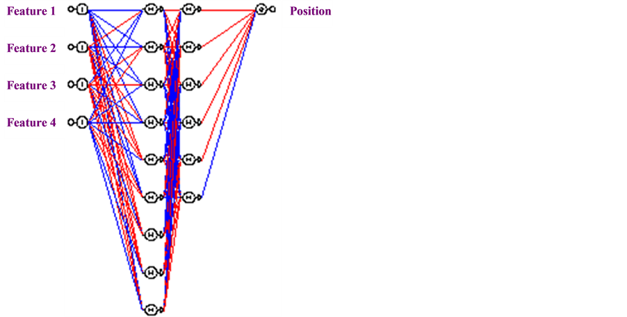
Figure 1. Neural network infrastructure.
Weight Elimination Algorithm is used to carry out weight decay process. It minimizes a modified error function which is formed by adding a penalty, liability or cost term to the original error function of the used algorithm [11] .
The liability variable in weight decay penalizes large weights, as it causes weights under consideration to converge to smaller absolute values. Large weights can negatively affect generalization according to their position in the network. If the weights with large values are between input layer and hidden layer, they can result in the output function to be too rough, possibly with near discontinuities. However, if they lie between the hidden layer and the output layer, they can result in wild outputs beyond the range of the data. Hence, large weights can cause excessive variance of the output and instability of the neural structure, as their values and instability will be outside the range of the output activation function. Weights size is very important and in some cases will have more effect than the number of weights in determining generalization.
Weight elimination mathematical representation is based on Ridge regression principles, whereby it describes the dynamic changes in neural network convergence through error functions. The overall weight elimination error function is presented by Equation (3), and it consists of two parts [12] [13] :
I. Initial error function described by Equation (4).
II. Penalty error function described by Equation (5)
 (3)
(3)
 (4)
(4)
 (5)
(5)
where;
 : The combined overhead function that includes the initial overhead function,
  and the weight-elimination term
 .
.
 : The weight-reduction factor.
 : Represents the individual weights of the neural network model.
 : A scale parameter computed by the WEA.
 : The desired Output: It represents the wanted position as a function of the four used features, as indicated in Figure 1, Table 1 and Table 2.
 : The actual Output: It represents the actual position, as a function of the four used features, as indicated in Figure 1, Table 1 and Table 2.
The dynamic weight changes is calculated through a modified version of the gradient descent algorithm as shown in equation (6)
 (6)
(6)
where;
 : The Learning Rate (between 0 and 1)
The parameter,  , is a scale parameter computed by the WEA, and chosen to be the smallest weight from the last epoch or set of epochs to force small weights to zero.
  guides the computing algorithm to find solutions with either fewer large weights or many small weights, depending on the
  values small or large.
Two clear cases can be realized:
Case 1: (7)
(7)
Here the algorithm needs to drive the weights values down and obtain small weights in large numbers.
Case 2: (8)
(8)
Here the algorithm needs to keep large weights in small numbers.
The error sum is carried out over all training examples and overall output nodes, with the initial error representing the complexity of the network as a function of the weight magnitude, which is relative to the scale parameter . The weight factor
 , determines the importance of the network complexity with respect to network performance over training sets, and can be adjusted during training and computed from equation (9).
 (9)
(9)
where;  is a scaling factor and can be set to 1,
  is multiplication constant, and
  is the ratio of correctly classified patterns from testing sets over the overall number of patterns.
  dynamically responds to
  changes, so when
  increases, so does
 , which leads to more contributions by
  in driving small weights towards zero to further increase generalization. However, when
  decreases, it will result in
  approaching a very small value, hence, suppressing the contribution by
  to the overall error expression and the neural structure would be at a bad state.
The role of the weight-reduction factor is to determine the relative importance of the weight-elimination term. Larger values of  push small weights to further reduce their size. Small values of
  will not affect the network. The choice of
  should be optimized such that it is not too large or too small. Too values of
  will result in fast decay of small weights, and too small values of
  will eliminate the process of pruning.
Selecting the stop point is critical to avoid over fitting and over pruning. When performance is poor, corresponding connections to weaker weights are removed, which will lead to redundant weights. To remove a weight, the algorithm, also looks at the relationship between , and when the relationship leads to
  becoming very small, weights are both driven to smaller values and removed. Weight Elimination Algorithm (WEA) is a bidirectional Bottom-Up, Top-Down pruning algorithm, starts with a simple, then complex network and drives unnecessary weights during training towards zero.
Preprocessing of the used training sets is carried out as follows:
1) Statistical Data Transformation (SDT) and Data Clustering (DC);
2) Each selected feature is a function of multi correlated variables that contribute to the positioning of the data record within the dataset.
The position of each record within a data set is a function of the correlation between the four features and between each record and the next one and the one before. To achieve correct and reliable analysis showing the disparity due to dominant pattern effect, the same neural structure is used for individual and joined patterns. The designed network needed to be complex as after few trials with simple designs and small number of nodes, the network did not converge with very high Mean Squared Error (MSE) [14] [15] .
3. Results
Figure 2 and Figure 3 show initial statistical representation of the features in both dataset 1 and dataset 2. Table 3 and Table 4 show the classified and predicted data using WEA.
Table 3. Predicted dataset 1 as a function of training datasets 1 and 2.
Table 4. Predicted dataset 1 as a function of training datasets 1 and 2.
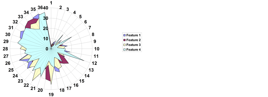
Figure 2. Dataset 1 features spread.
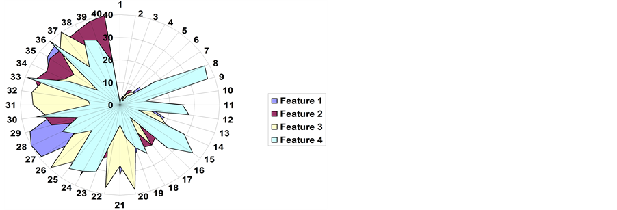
Figure 3. Dataset 2 features spread.
The approach for this work included three elements:
1) Collecting and pre-processing data to represent ranking or position of data records in each of the datasets;
2) Selecting an appropriate neural network algorithm to uncover the dominant pattern;
3) Correlating both data selection to the dynamics of the selected neural system.
Training of the designed neural network structure is carried out using three different sets:
I. Dataset 1;
II. Dataset 2;
III. Combined datasets 1 & 2.
4. Discussion
From Figure 2 and Figure 3, it is deduced that even though both datasets belong to the same general parent category, with exactly same rules applied to produce the sets and with many general common features in between them, dataset 2 seems to possess an abnormal spread that goes beyond the expected signature of the parent dataset that produced both sets.
Testing of the system for generalization, classification, and prediction, is carried out using both dataset 1 and dataset 2. This approach together with WEA, guarantee uncovering of which dataset is dominant as a result of the neural network output when either dataset is tested against all three permutations or sets, as shown in Table 3 and Table 4, while Table 5 summarizes and provides an evidence that dataset 2 is dominant as it dominates the training, testing process and the results obtained for dataset 1, whenever both datasets are either present in training or testing. Dataset 1 shown to be recessive with no effect on the way system behaves.
Table 5 is transformed in logic table presented in Table 6. From Table 6, it is clear that dataset 1 has no effect on dataset 2, but only on itself, as a perfect prediction and classification match for dataset 1 occurs when
Table 5. Pattern matching.
Table 6. Logical representation: pattern matching.
dataset 1 is used for both training and testing. For dataset 2, the table shows that whenever it is present in the training, alone or in combination with dataset 1, the system classifies accurately for either dataset 1 or the combined datasets 1 & 2. This is a solid proof that dataset 2 plays the dominant pattern with dataset 1 as the recessive pattern, which supports the initial plots in Figure 2 and Figure 3 regarding their initial characteristics.
Looking back at Table 3 and Table 4, it is realized that the mutation and disturbance in the results obtained for dataset 1 by dataset 2 when dataset 1 is used for training than the mutation in the results for dataset 2 by dataset 1 when dataset 1 is used for training. Such evidence goes along way to show the superior effect of dataset 2 on dataset 1 and on the combined sets.
From Table (6), three logical relationships can be represented:
1. (10)
(10)
2. (11)
(11)
3. (12)
(12)
It is noticed from the logical expressions that {a} occurs only once as a positive logic, but {b, c} occurs twice as positive logic with {a} in both cases in negation status. This further supports the dominant pattern effect with mutation consequences on dataset 1 or pattern {a}. Now, considering the dynamics of WEA, it is clear that the presence of dominating pattern affected and displaced the weight elimination process, whereby, excessive variance is caused when prediction and classification of dataset 1 is carried out after the neural structure is subjected to the influence to dataset 2. This dominating pattern affected weight distribution and ability of the system to identify the pattern associated with dataset 1, with total ability to perfectly reproduce the pattern associated with dataset 2 even when both datasets are used for training.
From Table 3 and Table 4, it is clear that dataset 1 has 2 matches out of 6 trials, and dataset 2 has 4 matches out of 6 trials, this gives:
 (13)
(13)
 (14)
(14)
 (15)
(15)
These results mean,
Since  has some contribution to the value, then
  both dataset 1 and dataset 2 share some common properties, but both did not originate from the same place, neither they are subsets of a larger dataset, hence, the domination of dataset 2 through its pattern.
If both datasets do not hold similar properties or been processed using similar features, then one of them should have Zero contribution to expression in (15).
If both datasets have equal contribution with no one pattern dominates, then it is expected that each one would have a 50% contribution value to the total pattern recognition.
If both datasets have no common features and not subsets of an original set, then it is expected that one of them would have Zero contribution with the other having 100% contribution value.
From above, we deduce the expression in (16) and (17):
 (16)
(16)
 (17)
(17)
This approach can be used to detect intruding and out of place datasets and the ones that do not belong to the general characteristics of the prescribed behavior of collection of datasets. Hence, it can be used as a filter and isolator which detects and removes datasets that suffer damage or that might have damaging effect on the overall system. Also, it can be used to analyze change in patterns and their effect on the rest of the holding main matrix.
Figure 4 shows the Mean Squared Error (MSE), computed for the same neural structure with training datasets:
I: Dataset 1;
II: Dataset 2;
III. Combined datasets 1 and 2.
It is evident that when dataset 2 has larger MSE compared to dataset 1, however, the interesting result is when both datasets are used for training, the MSE value dramatically increased. This behavior is consistent with the effect that dataset 2 has on the system dynamics and on dataset 1, where it unbalances the system due to its dominance and mutation properties [14] [15] .
5. Conclusions
This work proved a hypothesis that a dominant pattern would negatively affect the performance of a neural based pattern recognition system and would influence its operational behavior and dynamics in terms of its capabilities to classify, predict, and generalize.
Classification and prediction results of the WEA-BP showed clear dominance for dataset 2 on dataset 1. Such negative effect of dataset 2 through its pattern representation affected the weight elimination process and its corresponding weight change dynamics with subsequent mutation to the obtained results for dataset 1.
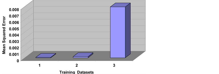
Figure 4. Mean squared error as a function of training datasets.
It is proved in this work that a neural network algorithm converges to the dataset with the most dominant effect. Such feature might be considered a good one, but on the contrary, if one or more dataset dominated the neural network behavior, then its pattern recognition, classification, and prediction would become deviated and unbalanced.
These findings in the research can be utilized to uncover foreign and hostile datasets and analyze their effects. Also, it can be a good approach to modify preprocessing techniques that will produce such dominant patterns.
Cite this paper
Mahmoud ZakiIskandarani, (2015) Disparity in Intelligent Classification of Data Sets Due to Dominant Pattern Effect (DPE). Journal of Intelligent Learning Systems and Applications,07,75-86. doi: 10.4236/jilsa.2015.73007
References
- 1. Belghinia, N., Zarghilib, A., Kharroubic, J. and Majdad, A. (2012) Learning a Backpropagation Neural Network with Error Function Based on Bhattacharyya Distance for Face Recognition. International Journal of Image, Graphics and Signal Processing, 4, 8-14.
http://dx.doi.org/10.5815/ijigsp.2012.08.02 - 2. Wilamowski, B.M. and Yu, H. (2010) Neural Network Learning without Backpropagation. IEEE Transactions on Neural Networks, 21, 1793-1803. http://dx.doi.org/10.1109/TNN.2010.2073482
- 3. Subrahmanya, N. and Yung, C.S. (2010) Constructive Training of Recurrent Neural Networks Using Hybrid Optimization. Neurocomputing, 73, 2624-2631.
http://dx.doi.org/10.1016/j.neucom.2010.05.012 - 4. Puma-Villanuevaa, W.J., Santos, E.P. and Zuben, F.J.A. (2012) Constructive Algorithm to Synthesize Connected Feedforward Neural Networks. Neurocomputing, 75, 14-32.
http://dx.doi.org/10.1016/j.neucom.2011.05.025 - 5. May, P., Zhou, E. and Lee, C.W. (2014) Improved Generalization in Recurrent Neural Networks Using the Tangent Plane Algorithm. International Journal of Advanced Computer Science and Applications, 5, 118-126.http://dx.doi.org/10.14569/IJACSA.2014.050317
- 6. Ahmed, S.U., Shahjahan, M.D. and Kazuyuki, M. (2011) A Limpel-Ziv Complexity Based Neural Network Pruning Algorithm. International Journal of Neural Systems, 21, 427-441.
http://dx.doi.org/10.1142/S0129065711002936 - 7. Bavafaye Haghighia, E., Palm, G., rahmati, M. and Yazdanpanahc, M.J. (2015) A New Class of Multi-Stable Neural Networks: Stability Analysis and Learning Process. Neural Networks, 65, 53-64.
http://dx.doi.org/10.1016/j.neunet.2015.01.010 - 8. Nie, X. and Zheng, W.X. (2015) Multistability of Neural Networks with Discontinuous Non-Monotonic Piecewise Linear Activation Functions and Time-Varying Delays. Neural Networks, 65, 65-70.
http://dx.doi.org/10.1016/j.neunet.2015.01.007 - 9. Wright Shrestha, S.B. and song, Q. (2015) Adaptive Learning Rate of SpikeProp Based on Weight Convergence Analysis. Neural Networks, 63, 185-198.
http://dx.doi.org/10.1016/j.neunet.2014.12.001 - 10. Li, X., Gong, X., Peng, X. and Peng, S. (2014) SSiCP: A New SVM Based Recursive Feature Elimination Algorithm for Multiclass Cancer Classification. International Journal of Multimedia and Ubiquitous Engineering, 9, 347-360.http://dx.doi.org/10.14257/ijmue.2014.9.6.33
- 11. Qingsong, Z., Jiaqiang, E., Jinke, G., Lijun, L., Tao, C., Shuhui, W. and Guohai, J. (2014) Functional Link Neural Network Prediction on Composite Regeneration Time of Diesel Particulate Filter for Vehicle Based on Fuzzy Adaptive Variable Weight Algorithm. Journal of Information & Computational Science, 11, 1741-1751.http://dx.doi.org/10.12733/jics20103209
- 12. May, P., Zhou, E. and Lee, C.W. (2013) A Comprehensive Evaluation of Weight Growth and Weight Elimination Methods Using the Tangent Plane Algorithm. International Journal of Advanced Computer Science and Applications, 4, 149-156. http://dx.doi.org/10.14569/IJACSA.2013.040621
- 13. Ennett, C.M. and Friz, M. (2003) Weight-elimination Neural Networks Applied to Coronary Surgery Mortality Prediction. Information Technology in Biomedicine. IEEE Transactions on Information Technology in Biomedicine, 7, 86-92. http://dx.doi.org/10.1109/TITB.2003.811881
- 14. Lalis, J.T., Gerardo, B.D. and Byun, Y. (2014) An Adaptive Stopping Criterion for Backpropagation Learning in Feedforward Neural Network. International Journal of Multimedia and Ubiquitous Engineering, 9, 149-156.http://dx.doi.org/10.14257/ijmue.2014.9.8.13
- 15. Iskandarani, M.Z. (2014) A Novel Approach to System Security Using Derived Odor Keys with Weight Elimination Neural Algorithm (DOK-WENA). Transactions on Machine Learning and Artificial Intelligence, 2, 20-31.http://dx.doi.org/10.14738/tmlai.22.138