Journal of Intelligent Learning Systems and Applications
Vol.5 No.1(2013), Article ID:27932,10 pages DOI:10.4236/jilsa.2013.51001
Linear and Nonlinear Trading Models with Gradient Boosted Random Forests and Application to Singapore Stock Market*
![]()
Department of Electrical and Computer Engineering, National University of Singapore, Singapore, Singapore.
Email: elewqg@nus.edu.sg
Received October 1st, 2012; revised November 6th, 2012; accepted November 13th, 2012
Keywords: Stock Modeling; Scoring Technique; Least Square Technique; Random Forest; Gradient Boosted Random Forest
ABSTRACT
This paper presents new trading models for the stock market and test whether they are able to consistently generate excess returns from the Singapore Exchange (SGX). Instead of conventional ways of modeling stock prices, we construct models which relate the market indicators to a trading decision directly. Furthermore, unlike a reversal trading system or a binary system of buy and sell, we allow three modes of trades, namely, buy, sell or stand by, and the stand-by case is important as it caters to the market conditions where a model does not produce a strong signal of buy or sell. Linear trading models are firstly developed with the scoring technique which weights higher on successful indicators, as well as with the Least Squares technique which tries to match the past perfect trades with its weights. The linear models are then made adaptive by using the forgetting factor to address market changes. Because stock markets could be highly nonlinear sometimes, the Random Forest is adopted as a nonlinear trading model, and improved with Gradient Boosting to form a new technique—Gradient Boosted Random Forest. All the models are trained and evaluated on nine stocks and one index, and statistical tests such as randomness, linear and nonlinear correlations are conducted on the data to check the statistical significance of the inputs and their relation with the output before a model is trained. Our empirical results show that the proposed trading methods are able to generate excess returns compared with the buy-and-hold strategy.
1. Introduction
No matter how difficult it is, how to forecast stock price accurately and trade at the right time is obviously of great interest to both investors and academic researchers. The methods used to evaluate stocks and make investment decisions fall into two broad categories—fundamental analysis and technical analysis [1]. Fundamentalist examines the health and potential to grow a company. They look at fundamental information about the company, such as the income statement, the balance sheet, the cash-flow statement, the dividend records, the news release, and the policies of the company. Technical analysis, in contrast, doesn’t study the value of a company but the statistics generated by market motions, such as historical prices and volumes. Unfortunately none of them will always work due to the certain randomness and non-stationary behavior of the market. Hence, an increasing number of studies have been carried out in effort to construct an adaptive trading method to suit the nonstationary market. Soft Computing is becoming a popular application in prediction of stock price. Soft computing methods exploit quantitative inputs, such as fundamental indicators and technical indicators, to simulate the behavior of stock market and automate market trend analysis.
One method is Genetic Programming GA. Dempster and Jones [2] use GP and build a profitable trading system that consists of a combination of multiple indicator-based rules. Another popular approach is Artificial Neural Network (ANN). Generally, an ANN is a multilayered network consisting of the input layer, hidden layer and output layer. One of the well-recognized neural network models is the Back Propagation (BP) or Hopfield network. Sutheebanjard and Premchaiswadi [3] use a BPNN model to forecast the Stock Exchange of Thailand Index (SET Index) and experiments show that the systems work with less than 2% error. Vincenzo and Michele [4] compare different architectures of ANN in predicting the credit risk of a set of Italian manufacture companies. They conclude that it is difficult to produce consistent results based on ANNs with different architectures. Vincenzo and Vitoantonio [5] use ANN model based on genetic algorithm to forecast the trend of a Forex pair (Euro/USD). The experiments show that the trained ANN model can well predict the exchange rate of three days. Vincenzo [6] compare ANN model with ARCH model and GARCH model in predicting exchange rate of Euro/USD. It is found that ARCH and GARCH models can produce better results in predicting the dynamics of Euro/USD. An extension of ANN is Adaptive Neuro-Fuzzy Inference System (ANFIS) [7]. ANFIS is a combination of neural networks and fuzzy logic, which, introduced by Zadeh [8], is able to analyze qualitative information without precise quantitative inputs. Agrawal, Jindal and Pillai [9] propose momentum analysis based on stock market prediction using ANFIS and the success rate of their system is around 80% with the highest 96% and lowest 76%.
In addition, some weight adjustment techniques are also developed to select trading rules adaptively. Bengtsson and Ekman [10] discuss three weighing techniques, namely Scoring technique, Least-Squares Technique and Linear Programing Technique. All the three techniques are used to dynamically adjust the weights of the rules so that the system will act according to the rules that perform best at the moment. The model is tested on Stockholm Stock Exchange in Sweden. As a result, it is able to consistently generate risk-adjusted returns.
Instead of finding out the weighting of predictors, Decision Tree [11] adopts an alternative approach by identifying various ways of splitting a data set into branchlike segments. Decision Tree is further improved by the Random Forest algorithm [12], which consists of multiple decision trees. Random forest is proven to be efficient in preventing over-fitting. Maragoudakis and Serpanos [13] apply random forest to stock market predictions. The portfolio budget for their proposed investing strategy outperforms the buy-and-hold investment strategy by a mean factor of 12.5% to 26% for the first 2 weeks and from 16% to 48% for the remaining ones.
Besides soft computing methods which use past data to forecast future trend, there is an alternative area of study which doesn’t predict the future at all but only follow the historical trend. That is known as Trend-Following (TF). Fong and Tai [14] design a TF model with both static and adaptive versions. Both yield impressive results: monthly ROI is 67.67% and 75.63% respectively for the two versions.
This paper presents various trading models for the stock market and test whether they are able to consistently generate excess returns from the Singapore Exchange (SGX). Instead of conventional ways of modeling stock prices, we construct models which relate the market indicators to a trading decision directly. Furthermore, unlike a reversal trading system or a binary system of buy and sell, we allow three modes of trades, namely, buy, sell or stand by, and the stand-by case is important as it caters to the market conditions where a model does not produce a strong signal of buy or sell. Linear trading models are firstly developed with the scoring technique which weights higher on successful indicators, as well as with the Least Squares technique which tries to match the past perfect trades with its weights. The linear models are then made adaptive by using the forgetting factor to address market changes. Because stock markets could be highly nonlinear sometimes, the decision trees with the Random Forest method are finally employed as a nonlinear trading model [15]. Gradient Boosting [16,17] is a technique in the area of machine learning. Given a series of initial models with weak prediction power, it produces a final model based on the ensemble of those models with iterative learning in gradient direction. We apply Gradient Boosting to each tree of Random Forest to form a new technique—Gradient Boosted Random Forest for performance enhancement. All the models are trained and evaluated on nine stocks and one index, and statistical tests such as randomness, linear and nonlinear correlations are conducted on the data to check the statistical significance of the inputs and their relation with the output before a model is trained. Our empirical results show that the proposed trading methods are able to generate excess returns compared with the buy-and-hold strategy.
The rest of this paper is organized as: the input selection is presented in Section 2. In Section 3, we describe the linear model and adaptation. The decision tree and random forest are given in Section 4. The new method— gradient boosted random forest—is presented in Section 5. The Section 6 shows the simulation studies and the conclusion is in the last section.
2. Input Selection
2.1. Basic Rules
The model is built upon a fixed set of basic rules. All the rules use historical stock data as inputs and generate “buy”, “sell” or “no action” signals. Rules [18] adopted in this paper are some popular, wide-recognized and published rules as summarized below.
• Simple Moving Average (SMA). SMA is the average price of a stock over a specific period. It smoothes out the day-to-day fluctuations of the price and gives a clearer view of the trend. A “buy” signal is generated if the SMA changes direction from downwards to upwards, and vice versa. In this paper, 5-day, 10-day, 20-day, 30-day, 60-day and 120-day SMAs are studied.
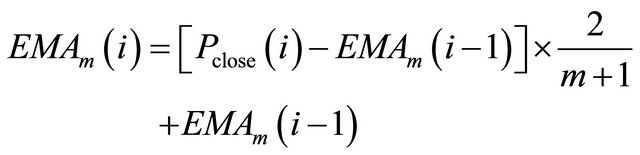
• Exponential Moving Average (EMA). EMA is similar to SMA, but EMA assigns higher weight to the more recent prices. Thus, EMA is more sensitive to recent prices. The expression is:
 (1)
(1)
where ![]() is the number of days in one period,
is the number of days in one period,  is the closing price of day
 ,
,  is the m-day EMA of day
 ,
,  is the mday EMA of the previous day.
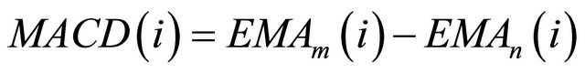
• Moving Average Convergence/Divergence (MACD). MACD measures the difference between a fast (shortperiod) and slow (long-period) EMA. When the MACD is positive, in other words, when the shortperiod EMA crosses over the long-period EMA, it signals upward momentum, and vice versa. Two signal lines are used—zero line and 9-day SMA. A “buy” signal is generated if the MACD moves up and crosses over the signal line, and vice versa. The expression is:
 (2)
(2)
where![]() . The most common moving average values used in the calculation are the 26-day and 12- day EMA, so m = 12 and n = 26.
. The most common moving average values used in the calculation are the 26-day and 12- day EMA, so m = 12 and n = 26.
• Relative Strength Index (RSI). RSI signals overbought and oversold conditions. Its value ranges from 0 to 100. A reading below 30 suggests an oversold condition and thus a “buy” signal is generated; a reading above 70 usually suggests an overbought condition and thus a “sell” signal is generated; take “no action”, otherwise.
• Stochastics Oscillator. Stochastics Oscillator is a wellrecognized momentum indicator. The idea behind this indicator is that price close to the highs of the trading period signals upward momentum in the security, and vice versa. It’s also useful to identify overbought and oversold conditions. It contains two lines—the %K line and the %D line. The latter is a 3-day SMA of the former. Its value ranges from 0 to 100. A “buy” signal is generated if the %D value is below 20; a “sell” signal is generated if the %D value is above 80; take “no action”, otherwise.
• Bollinger Bands. Bollinger Bands are used to identify overbought and oversold conditions. It contains a center line and two outer bands. The center line is an exponential moving average; the outer bands are the standard deviations above and below the center line. The standard deviations measure the volatility of a stock. It signals oversold when the price is below the lower band and thus a “buy” signal is generated; it signals overbought when the price is above the upper band and thus a “sell” signal is generated; take “no action”, otherwise.
• Accumulation/Distribution Line. A/D line measures volume and the flow of money of a stock. Many times before a stock advances, there will be period of increased volume just prior to the move. When the A/D Line forms a positive divergence—when the indicator moves higher while the stock is declining—it gives a bullish signal. Therefore, a “buy” signal is generated when the indicator increases while the stock is declining; a “sell” signal is generated when the indicator decreases while the stock is rising; take “no action”, otherwise. The expression is:
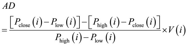 (3)
(3)
where  is the lowest price of day
 ,
,  is the highest price of day
 ,
,  is the open price of day
 , and
, and  is the trading volume of day
 .
.
2.2. Statistics Tests
Statistical tests are carried out for input selection. Firstly, it is useful to test whether the input data are random or not. If the input data are random, it is rather difficult to make predictions based on random data. Secondly, it is necessary to test whether the input data are related to the output data. If a correlation between input data and output data cannot be found, the output of the model may be randomly generated instead of being a result of the input data. Therefore, only when the inputs are statistically significant, they are used to build models.
Three statistical tests are introduced—the WilcoxonMann-Whitney test for the randomness of signs, the Durbin-Watson Test for linear interaction effect between input and output, and the Spearman’s correlation [19] for nonlinear correlation between input and output.
• The Wilcoxon-Mann-Whitney Test. This test performs a test of the null hypothesis that the occurrence of “+” and “−” signs in a data set is not random, against the alternative that the “+” and “−” signs comes in random sequences. Mathematically, the test works in the following way. Let n1 be the number of − or + signs, whichever is larger and n2 be number of opposite signs. N = n1 + n2. From the order/indices of the signs in the data sequence, the rank sum R of the smallest number of signs is determined. Let  =
= . The minimum of R and
  is used as the test statistics. In this project, it is desired to test whether the input data are random or not. If input data are already random, it is rather difficult to make predictions based on random input. Note that the test only takes care of “+” and “−” signs. Thus, for any sequence of data, a sequence of “+” and “−” signs can be easily generated by taking the difference of two consecutive data points.
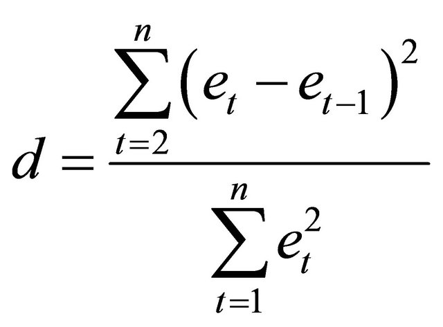
• Durbin-Watson Test. This test is used to check if the residuals are uncorrelated, against the alternative that there is autocorrelation among them. This test is based on the difference between adjacent residuals and is given by
 (4)
(4)
where et is the regression residual for period t, and n is the number of time periods used in fitting the regression model. Correlations are useful because they can indicate a predictive relationship that can be exploited in practice. In this project, it is desired to find the interactive effect of the input data R on the output data Y. The error terms et are the residuals of the linear regression of the responses in Y on the predictors in R.
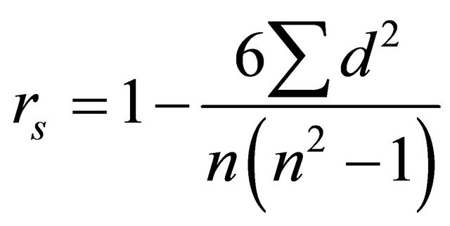
• Spearman’s Corrections. Previously, the Durbin-Watson test is used to measure the strength of the linear association between two variables. However, it is less appropriate when the points on a scatter graph seem to follow a curve or when there are outliers (or anomalous values) on the graph [19]. Spearman’s correlation coefficient measures nonlinear correlation. To find the Spearman’s correlation coefficient of two data sequences X and Y, first rank each data vector in either ascending or descending order. Then calculate the Spearman’s correlation coefficient by the following formula:
 (5)
(5)
where n is the number of data pairs, and d = rank xi - rank yi.
3. Linear Model and Adaptation
3.1. Trading Method
A fixed set of the basic rules are used as the inputs to our models. Each basic rule returns an integer to represent its recommended trading actions—“1” represents a “buy” signal; “−1” represents a “sell” signal; and “0” represents “no action”.
The model works in two steps—training and testing. During the training period, each rule is evaluated on a set of the known historical data and assigned a certain weight using some rule-weighting algorithms. Two weighting algorithms are proposed and described later.
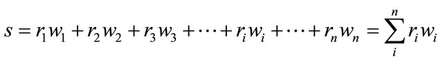
After training is the testing period, during which the model predicts trading decisions based on unknown data and its performance is evaluated. On a daily basis, the model collects trading recommendations—“1” or “−1” or “0”—generated by those rules. These recommendations are then fed into a weighting filter. In the weighting filter, each rule’s recommendation is multiplied by its corresponding weight, which is previously determined by the training process. Finally, the weighted rules are summed up as an overall weighted recommendation. The greater the value of the sum, the stronger the recommendation is. The weighted recommendation is interpreted as “buy”, or “sell”, or “no action” depending on the strength of the recommendation and whether the stock is currently owned or not. Mathematically,
 (6)
(6)
where s is the final trading decision, ri is the output value of each rule ( ri takes the value 1, or −1, or 0), wi is the adjusted weight of each rule obtained from the training period.
A larger s indicates a stronger signal and thus the system is more confident about the derived trading decision. Therefore, only when the resulting signal is above a certain threshold, it is regarded as a “buy” signal; similarly, only when it is below a certain threshold, it is regarded as a “sell” signal; if it is between the upper and lower thresholds, “no action” is taken.
3.2. Rule-Weighting Algorithms
At the beginning all weights are equal with a value of 0. As already mentioned, the weight of each rule is adjusted during training. The higher the weight, the stronger the trading recommendation generated by the rule. After adjusting the weights, bad rules will end up with small or even negative weights. Two rule-weighting algorithms— the scoring and the least-squares techniques are described as follows.
• Scoring Technique: The scoring technique grades the rules according to how well they have performed. During the training period whenever a rule gives a “buy” or “sell” recommendation, the weight of the rule is adjusted—weight is increased by 1 if the recommendation is correct; otherwise, weight is decreased by 1. “No action” signal doesn’t trigger weight adjustment. Here, a correct “buy” recommendation refers to the situation that the close price next day is a certain amount higher than the close price today when the recommendation is given; while a correct “sell” recommendation is similarly defined; and if none of the above is true, no recommendation is given.
• Least-Squares Technique: The second rule-weighting algorithm is the least-squares technique with the linear regression. Firstly, when it is known that the price is increased or decreased the next day during the training period, it is also known what trading action should be taken on that day. Secondly, the trading recommendations of each rule are also known. The least-squares technique is an algorithm that finds a set of weights that maps the trading recommendations by all the rules to the correct trading actions to be taken. Mathematically, if there are n rules and m training days in total,
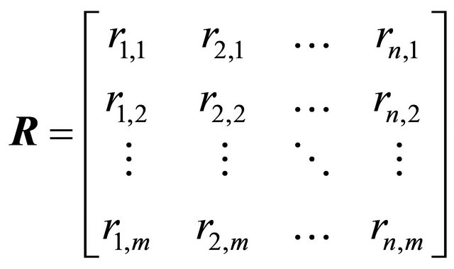
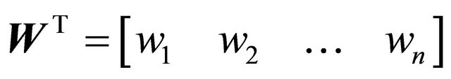
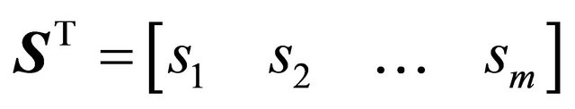
where R is an m×n matrix that stores the recommendations ri,j given by each rule every day, W is an n × 1 matrix that stores the weight of each rule wj. S is an m×1 matrix that stores the correct trading decision si which should be taken every day. si is determined by the following reasoning. On day i1) If price increases more than a threshold the next day, then the correct signal is “buy” and thus si = 1.
2) If price decreases more than a threshold the next day, then the correct signal is “sell” and thus si = –1.
3) If price only fluctuates within more than a threshold, the correct signal is “no action” and thus si = 0.
Ideally, S = RW. There are as many equations as the number of days in the training period, and n unknown variables—the weights for the n rules. With S and R known, if W can be solved, then W is the desired weights that can give correct signals. However, there are more training days than the number of rules and thus more equations than unknown variables, so the solution is over-specified. Thus, the objective now becomes to minimize the error e = S – RW. Define the cost function as
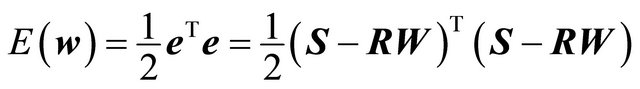 (7)
(7)
At the optimal point ,
,
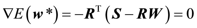 (8)
(8)
Thus,
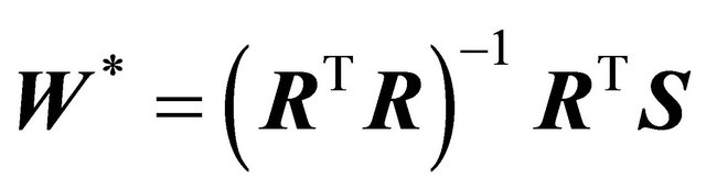 (9)
(9)
Hence, the least-squares technique finds the optimal weights to match the correct trading decisions as much as possible.
The Least-Squares technique can be further improved by the introducing nonlinear terms and forgetting factors. First, any two of the rules are combined together by multiplication to form a new “rule”—the non-linear term. Now the trading decision s becomes
 (10)
(10)
By introducing the forgetting factor, as its name suggests, more recent data have more influence on the final decision. Besides, this adaptive model is implemented by using the Recursive Least Squares algorithm, which updates the weight on a daily basis. Hence, Recursive Least Squares method doesn’t require the entire training data set for each iteration.
Every day, a new set of data comes in and the weights are updated based on the new set of data. The calculation is summarized below.

where ![]() is the forgetting factor with a value ranging from 0 to 1. Here
is the forgetting factor with a value ranging from 0 to 1. Here ![]() is set to be 0.95 in this paper.
is set to be 0.95 in this paper.
4. Decision Tree and Random Forest
4.1. Decision Tree
Unlike the previous trading models, which derive the final trading decision by summing up the weighted rules, decision tree [20] adopts a different approach to arrive at the final decision. As its name suggests, decision tree identifies various ways of splitting a data set into branchlike segments (Figure 1). These segments form a tree-like structure that originates with a root node at the top of the tree with the entire set of data. A terminal node, or a leaf, represents a value of the output variable given the values of the input variables represented by the path from the root to the leaf. A simple decision tree is illustrated below.
• Growing the tree: The goal is to build a tree that distinguishes a set of inputs among the classes. The process starts with a training set for which the target classification is known. For this project, we want to make trading decisions based on various indicators. In other words, the tree model should be built in a way that distinguish each day’s rule data to either “buy”, “sell” or “no action”. The input data set is split into branches. To choose the best splitting criterion at a node, the algorithm considers each input variable. Every possible split is tried and considered, and the best split is the one which produces the largest decrease in diversity of the classification label within each partition. The process is continued at the next node and, in this manner, a full tree is generated.
• Pruning the tree: For a large data set, the tree can grow into many small branches. In that case, pruning is carried out to remove some small branches of the tree in order to reduce over-fitting. During the training process, the tree is built starting from the root node where there is plenty of information. Each subsequent split has smaller and less representative information with which to work. Towards the end, the information may reflect patterns that are only related to certain training records. These patterns can become meaningless and sometimes harmful for prediction if you try to extend rules based on them to larger populations. Therefore, pruning effectively reduces overfitting by removing smaller branches that fail to generalize.
4.2. Random Forest
Random forest [13] , as its name suggests, is an ensemble of multiple decision trees. For a given data set, instead of one single huge decision tree, multiple trees are planted as a forest. Random forest is proven to be efficient in preventing over-fitting. One way of growing such an ensemble is bagging [21]. The main idea is summarized below:
Given a training set D = {y, x}, one wants to make prediction of y for an observation of x.
1) Randomly select n observations from D to form Sample B-data sets.
2) Grow a Decision Tree of each B data set.
3) For every observation, each tree gives a classification, and we say the tree “votes” for that class. The final output classifier is the one with the highest votes.
In the process of growing a tree (step 2 above), randomly select a fixed-size subset of input variables instead of using all the input variables. The best split is used to split the tree. For example, if there are ten input variables, only select three of them at random for each decision split. Each tree is grown to the largest extent possible without pruning. Random selection of features reduces
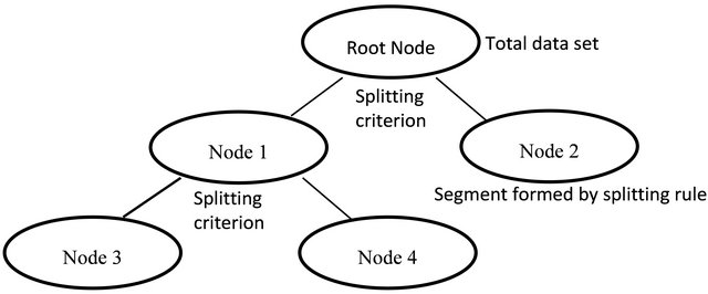
Figure 1. Decision tree.
correlation between any two trees in the ensemble and thus increases the overall predictive power.
In this project, the values of technical indicators are used as the input data set of the random forest and the output is the vector of percentages of votes for the trading actions for −1 (sell), 0 (no action) or 1 (buy).
Compared to other data mining technologies introduced before, Decision Tree and Random Forest algorithms have a number of advantages. Tree methods are nonparametric and nonlinear. The final results of using tree methods for classification or regression can be summarized in a series of logical if-then conditions (tree nodes). Therefore, there is no implicit assumption that the underlying relationships between the predictor variables and the target classes follow certain linear or nonlinear functions. Thus, tree methods are particularly well suited for data mining tasks, where there is often little knowledge or theories or predictions regarding which variables are related and how. Just like stock data, there are great uncertainties and unsure relationships between technical indicators and the desired trading decision.
5. Gradient Boosted Random Forest
5.1. Gradient Boosting
Gradient boosting is a technique in the field of machine learning. This technique was originally used for regression problems. With the help of loss function, classification problems can also be solved by this technique. This technique works by producing an ensemble of models with weak prediction power.
Suppose a training set of ,
,  ,
,  ,
,  and a differentiable loss function
 , and the iteration number M. Firstly, a model is initialized from:
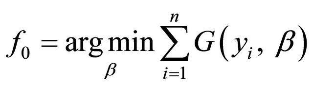 (11)
(11)
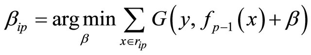
For the p-th iteration till p = M, calculate:
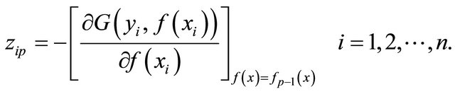 (12)
(12)
Let  be the number of terminal nodes of a decision tree. Correspondingly, the input space is divided into
  disconnected regions by the tree, which are represented as
 ,
,  ,
,  ,
,  at the p-th iteration. Then we can use the training data
 ,
,  ,
,  ,
,  to train a basic learner:
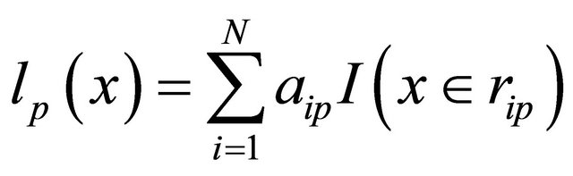 (13)
(13)
where  is the predicted value in region
 . The approximation
  can be expressed as:
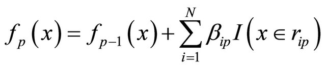 (14)
(14)
and,
 . (15)
5.2. Size of Trees
As mentioned above,  represents the number of leaves of decision trees. Hastie et al. [22] show that it works well when
 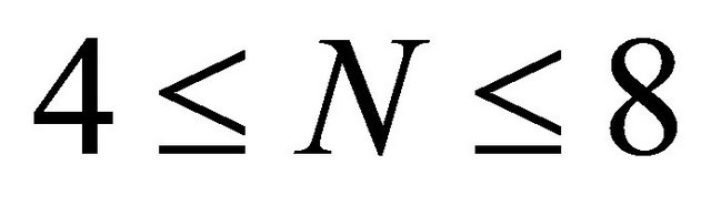 and the results will not change much when the
  is in this range. N beyond this range is not recommended.
5.3. Gradient Boosted Random Forest
Firstly, we set the size of the decision trees and create a random forest with equal size of its trees. Next, we set the iteration number for gradient boosting and apply it to each of the above trees. As a result, the random forest with each tree boosted is formed and called a gradient boosted random forest.
6. Simulation Studies
6.1. Data
This paper focuses on the Singapore stock market, and our simulation tests nine representative stocks traded on SGX as well as the Straits Times Index (STI) as a benchmark as listed in Table 1. In order to test how the proposed trading strategy performs in different economic sectors, the nine stocks are from various sectors of the Singapore economy. For all ten stocks, a set of five-year historical data ranging from September 1, 2005 to August 31, 2010 are studied, and the first three years’ data are used for training while the last two years for testing. Historical data are retrieved from Yahoo Finance (Singapore). Historical data provided here are daily data including daily open, close, high, low prices and volume. No pre-processing for changing the distribution of the classes is performed. In fact, different stocks have different distributions of classes. We use the real data to do
Table 1. List of stocks tested.
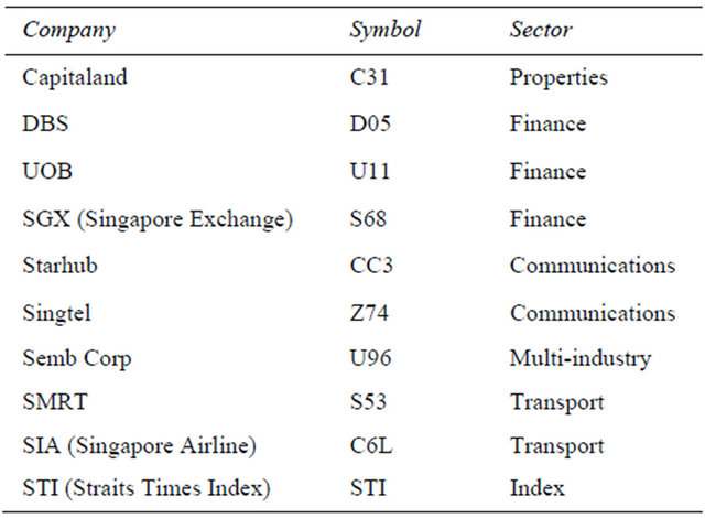
the experiment. Thus, the results are realistic without artificial distortion. Take the stock “Singtel” for example: the data have three classes: A, B and C. The corresponding distribution is A, 11.26%, B, 65.39% and C, 23.35%. We use the data directly in the experiment and no change for the distribution is done. This is true for all the stocks.
6.2. Statistical Tests Results
Before actually training any model, statistical tests are conducted. Firstly, Wilcoxon-Mann-Whitney test is applied on historical price, technical indicators and trading rules. As a result, the statistics show non-random data. Then the Durbin-Watson test is performed in order to find the interactive effect of the input data on the output data. However, little linear correlation is observed. Thus, Spearman’s Correlation Coefficients for input and output data are calculated and as a result, some nonlinear correlation can be found. Therefore, it is proved statistically that input data are not random and input and output are nonlinearly correlated. Now, it is meaningful to evaluate the modeling results.
6.3. Performance Evaluation
A trading strategy is typically evaluated by comparing to the “buy & hold” strategy, in which the stock is bought on the first day of the testing period and held all the time until the last day of testing period. At the beginning of the testing period, assume that we initially have $10,000 cash on hand. At the end of the testing period, all holding stocks are sold for cash.
In order to replicate the real world as close as possible, transaction cost must be taken into consideration. In Singapore, the transaction cost is around 0.34% [23]. To ensure fair evaluation, in the proposed trading method, cash is invested into risk free asset when it is not use to buy any stock [24].
6.4. Performance Test
For the techniques of Scoring and Least-Squares, we test the sensitivity of threshold. It is found that the performance is not changed obviously when different threshold values are adopted. However, when the threshold value is equal to 0.55, most cases can produce good results. In this regard, we use 0.55 as threshold value to proceed. For the techniques of Random Forest and Gradient Boosted Random Forest, we set the forest size as 50. Each tree will give a prediction and the final output will be based on the majority of the trees votes.
We applied each technique to each stock and obtained their wealth dynamics. Take the stock “Singtel” for example, and its wealth time responses over five techniques are shown in Figure 2.
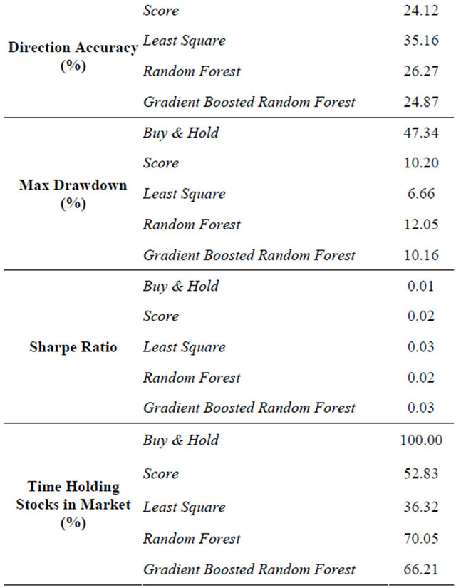
For investment performance evaluation, Table 2 shows the simulation results of the proposed trading methods— scoring, least squares, random forest and gradient boosted random forest—against the “buy & hold” strategy. The proposed trading methods are able to generate higher returns than the “buy & hold” strategy. On average, the gradient boosted random forest algorithm yields the highest total return followed by the random forest algorithm, scoring technique and the least-squares technique, while the “buy and hold” strategy makes a loss at −1.94%. Despite the positive results, the directional accuracy of the model is low, and the percent positive trade is lower than 50%.
From the Table 2, we can see that for the Gradient Boosted Random Forest, the total return of is 25.14%. The performance is slight better than the performance of Random Forest. The other two methods which are “Score” and “Least Square” produce worse results. This results show that using Gradient Boosted Random Forest can help gain more profit in the stock market than “buy & hold” strategy.
Although the system generates higher total returns, the directional accuracy is generally lower than 50%. As mentioned earlier, directional accuracy is only measured for “buy” and “sell” trading signals. In addition, there are
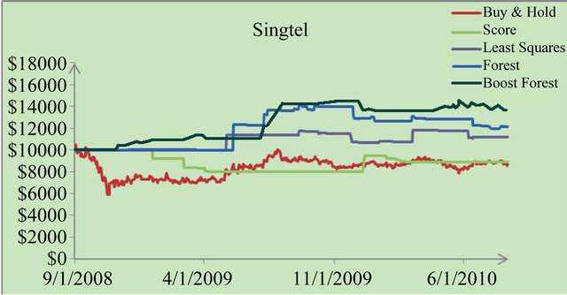
Figure 2. Wealth curve.
Table 2. Comparison results.
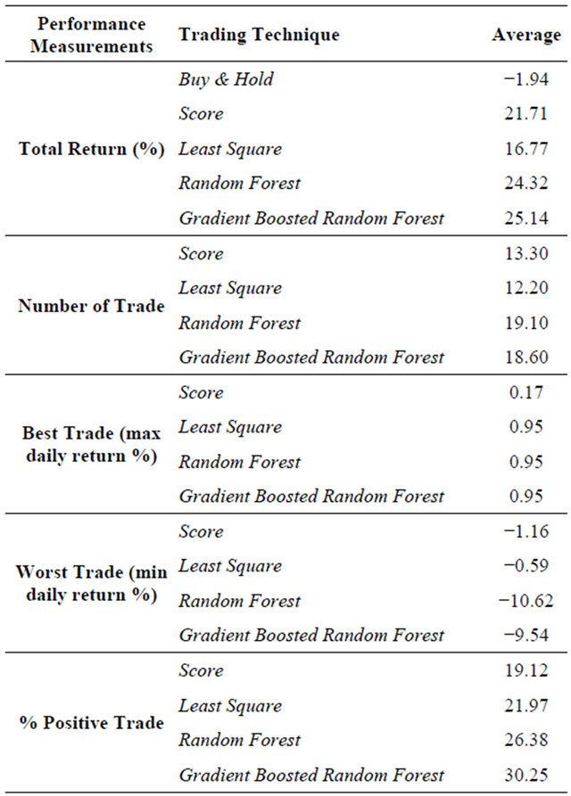
only 12 to 17 trading actions on average for a stock in the two years’ time and on most days no action is taken. The trading frequency is influenced by the threshold set for the system. If the threshold is high, only strong trading signals are put into effect.
Furthermore, fewer than half of the trades generate positive returns, however, the total return can be positive. It is due to the great increase in several trades. This is also reflected in the maximum drawdown.
Sharpe ratio measures the excess return per unit risk generated by the proposed trading method compared to investing into a risk free asset. Some of the ten stocks result in negative sharpe ratios. In other words, trading those two stocks fails to generate excess returns as compared to risk free asset.
In addition to five-year data, ten-year data of three stocks are evaluated—the training period is extended from two years to eight years while the testing period remains two years. Nevertheless, no obvious improvement is obtained. Comparisons between the linear model and the recursive nonlinear least squares model are also studied, but again no obvious improvement is found. The reason may be that making the algorithm too adaptive may over-fit the model. Besides, stock data itself are rather difficult to model.
7. Conclusion
This paper presents various trading models for the stock market and test whether they are able to consistently generate excess returns from the Singapore Exchange (SGX). Instead of conventional ways of modeling stock prices, we construct models which relate the market indicators to a trading decision directly. Furthermore, unlike a reversal trading system or a binary system of buy and sell, we allow three modes of trades, namely, buy, sell or stand by, and the stand-by case is important as it caters to the market conditions where a model does not produce a strong signal of buy or sell. Linear trading models are firstly developed with the scoring technique which weights higher on successful indicators, as well as with the least squares technique which tries to match the past perfect trades with its weights. Since stock markets could be highly nonlinear sometimes, the random forest method is then employed as a nonlinear trading model. Gradient boosting is a technique in the area of machine learning. Given a series of initial models with weak prediction power, it produces a final model based on the ensemble of those models with iterative learning in gradient direction. We apply gradient boosting to each tree of random forest to form a new technique—Gradient Boosted Random Forest—for performance enhancement. All the models are trained and evaluated and statistical tests such as randomness, linear and nonlinear correlations are conducted on the data to check the statistical significance of the inputs and their relation with the output before a model is trained. Our empirical results show that the proposed trading methods are able to generate excess returns compared with the buy-and-hold strategy. In particular, for the experimental data, the gradient boosted random forest yields highest total return with a value of 25.14%, followed by random forest whose total return is 24.32%, while the “buy and hold” strategy makes a loss at −1.94% every year.
REFERENCES
- R. D. Edwards, J. Magee and W. H. C. Bassetti, “Technical Analysis of Stock Trends, Chapter 1. The Technical Approach to Trading and Investing,” 9th Edition, CRC Press, Boca Raton, 2007, pp. 3-7.
- M. A. H. Dempster and C. M. Jones, “A Real-Time Adaptive Trading System Using Generic Programming,” Quan- titative Finance, Vo. 1, No. 4, 2001, pp. 397-413. doi:10.1088/1469-7688/1/4/301
- P. Sutheebanjard and W. Premchaiswadi, “Stock Exchange of Thailand Index Prediction Using Back Propagation Neural Networks,” 2nd International Conference on Computer and Network Technology, Bangkok, 23-25 April 2010.
- V. Pacelli and M. Azzollini, “An Artificial Neural Network Approach for Credit Risk Managemet,” Journal of Intelligent Learning Systems and Applications, Vol. 3, No. 2, 2011, pp. 103-112.
- V. Pacelli, V. Bevilacqua and M. Azzollini, “An Artificial Neural Network Model to Forecast Exchange Rates,” Journal of Intelligent Learning Systems and Applications, Vol. 3, No. 2, 2011. pp. 57-69.
- V. Pacelli, “Forecasting Exchange Rates: A Comparative Analysis,” International Journal of Business and Social Science, Vol. 3, No. 10, 2012, pp. 145-156.
- Wikipedia. http://en.wikipedia.org/wiki/Adaptive_neuro_fuzzy_inference_system
- A. La Zadeh, “Outline of a New Approach to the Analysis of Complex Systems and Decision Processes,” IEEE Transactions on Systems, Man and Cybernetics, Vol. 3, No. 1, 1973, pp. 28-44. doi:10.1109/TSMC.1973.5408575
- S. Agrawal, M. Jindal and G. N. Pillai, “Momentum Analysis Based Stock Market Prediction Using Adaptive Neuro-Fuzzy Inference System (ANFIS),” Proceedings of the International Multi Conference of Engineers and Computer Scientists, Hong Kong, 17-19 March 2010.
- M. Ekman and M. Bengtsson, “Adaptive Rule-Based Stock Trading: A Test of the Efficient Market Hypothesis,” MS Thesis, Uppsala University, Uppsala, 2004.
- J. M. Anthony, N. F. Robert, L. Yang, A. W. Nathaniel, and D. B. Steven, “An Introduction to Decision Tree Modeling,” Journal of Chemometrics, Vol. 18, No. 6, 2004, pp. 275-285. doi:10.1002/cem.873
- L. Breiman, “Random Forests,” Machine Learning Journal, Vol. 45, No. 1, 2001, p. 532.
- M. Maragoudakis and D. Serpanos, “Towards Stock Market Data Mining Using Enriched Random Forests from Textual Resources and Technical Indicators,” Artificial Intelligence Applications and Innovations IFIP Advances in Information and Communication Technology, Larnaca, 6-7 October 2010, pp. 278-286.
- S. Fong and J. Tai, “The Application of Trend Following Strategies in Stock Market Trading,” 5th International Joint Conference on INC, IMS and IDC, Seoul, 25-27 August 2009.
- Q.-G. Wang, J. Li, Q. Qin and S. Z. Sam Ge, “Linear, Adaptive and Nonlinear Trading Models for Singapore Stock Market with Random Forests,” Proceedings of 9th IEEE International Conference on Control and Automation, Santiago, 19-21 December 2011, pp. 726-731.
- J. H. Friedman, “Greedy Function Approximation: A Gradient Boosting Machine,” Technical Report, Stanford University, Stanford, 1999.
- J. H. Friedman, “Stochastic Gradient Boosting,” Technical Report, Stanford University, Stanford, 1999.
- Chart School, 2010. http://stockcharts.com/school/doku.php?id=chart_school:technical_indicators
- Schoolworkout Math, “Spearman’s Rank Correlation Coefficient,” 2011. http://www.schoolworkout.co.uk/documents/s1/Spearmans%20Correlation%20Coefficient.pdf
- J. M. Anthony, N. F. Robert, L. Yang, A. W. Nathaniel and D. B. Steven, “An Introduction to Decision Tree Modeling,” Journal of Chemometrics, Vol. 18, No. 6, 2004, pp. 275-285. doi:10.1002/cem.873
- L. Breiman, “Bagging Predictors,” Machine Learning, Vol. 26, No. 2, 1996, pp. 123-140. doi:10.1007/BF00058655
- Wikipedia. http://en.wikipedia.org/wiki/Adaptive_neuro_fuzzy_inference_system
- Fees: Schedules, DBS Vikers Online, 2010. http://www.dbsvonline.com/English/Pfee.asp?SessionID=&RefNo=&AccountNum=&Alternate=&Level=Public&ResidentType=
- Monetary Authority of Singapore, Financial DatabaseInterest Rate of Banks and Finance Companies, 2010. http://secure.mas.gov.sg/msb/InterestRatesOfBanksAndFinanceCompanies.aspx
NOTES
*This paper is an extended version of paper: Wang Qing-Guo, Jin Li, Qin Qin Shuzhi Sam Ge, “Linear, Adaptive and Nonlinear Trading Models for Singapore Stock Market with Random Forests”, The 9th IEEE International Conference on Control & Automation, Santiago, Chile, December 19-21, 2011.