Wireless Sensor Network
Vol.09 No.01(2017), Article ID:73525,15 pages
10.4236/wsn.2017.91001
Controlled Mobility Time Synchronization for WSNs
Gopal Chand Gautam, Narottam Chand Kaushal
Department of Computer Science & Engineering, National Institute of Technology Hamirpur, Hamirpur, India

Copyright © 2017 by authors and Scientific Research Publishing Inc.
This work is licensed under the Creative Commons Attribution International License (CC BY 4.0).
http://creativecommons.org/licenses/by/4.0/


Received: December 1, 2016; Accepted: January 14, 2017; Published: January 17, 2017
ABSTRACT
One of the important aspects in wireless sensor networks is time synchronization. Many applications such as military activity monitoring, environmental monitoring and forest fire monitoring require highly accurate time synchronization. Time synchronization assures that all the sensor nodes in wireless sensor network have the same clock time. It is not only essential for aforementioned applications but it is mandatory for TDMA scheduling and proper duty cycle coordination. Time synchronization is a challenging problem due to energy constraints. Most of the existing synchronization protocols use fixed nodes for synchronization, but in the proposed synchronization, algorithm mobile nodes are used to synchronize the stationary nodes in the sensing field. In this paper, we propose a new time synchronization algorithm, named controlled mobility time synchronization (CMTS) with the objective to achieve the higher accuracy while synchronizing the nodes. The proposed approach is used in this paper to synchronize the nodes externally by using the mobile nodes. Simulation results exhibit that proposed controlled mobility time synchronization increases the synchronization precision and reduces the energy consumption as well as synchronization error by reducing the collisions and retransmissions.
Keywords:
Wireless Sensor Network, Time Synchronization, Mobility, Offset, Energy

1. Introduction
Revolutionary technological changes in the field of microelectronics and wireless communications have resulted in the emergence of wireless sensor networks (WSN). The network is composed of numerous motes equipped with miniature sensors. The advantageous features of these motes are low cost, small size, multi-functionality and mobility. In modern era, wireless sensor networks have grown in popularity and are being used in various applications such as target tracking surveillance, seismic sensing, environmental monitoring and biomedical health monitoring [1] . Wireless sensor networks stem from the fact that nodes have limited resources in terms of memory, bandwidth, computation power and energy, which leads to new design challenges.
In the recent past, many valuable researches have been conducted for time synchronization in WSNs [2] - [31] . The aim of the existing researches is to synchronize the nodes externally by using mobile node which is equipped with GPS to estimate the clock offset precisely. In large WSNs, nodes communicate with each other via multi-hop paths. To synchronize the nodes, using multi-hop communication accumulate synchronization error at each hop. In larger WSNs, performance and the information collected by the nodes will not provide the precise time of the event.
This paper proposes Controlled Mobility Time Synchronization (CMTS) technique for wireless sensor networks. Major objective of CMTS is to reduce the synchronization error besides energy consumption of the nodes by reducing the communication distance among nodes. CMTS also conserves the energy of the nodes by reducing the collisions. The proposed CMTS is analyzed by simulation and the results show that proposed algorithm dissipates less energy than TTS and TSPN [27] . Results also indicate that the MNTS achieves lower synchronization error than TTS and TPSN.
The rest of the paper is organized as follows: Section 2 presents related work; Section 3 describes the proposed mobile node model and mobile node based time synchronization; Section 4 contains the simulations and analysis; and finally we conclude the paper in Section 5.
2. Related Work
In WSNs, there exist many time synchronization protocols. Some of the protocols synchronize the nodes internally by placing the nodes on common notion of time and some synchronize externally by adjusting the clocks of the sensor nodes with global clock. But none of the existing protocols exploits the mobility of the node for time synchronization.
Wang et al. proposed two-hop time synchronization protocol (TTS) with the objective to decrease the synchronization overhead and to offer more precise network-wide synchronization [27] . TTS uses common node to reduce the communication range of reference node. TTS uses the sender-receiver approach where common node gets the time information from root node and common node further transfers the time message to its neighboring nodes. In this way, the multi-hop TSS is used to synchronize the nodes which are not within the communication range of root node.
Djenouri et al. [28] proposed fast distributed multi-hop relative time synchronization protocol and estimator for WSNs. These protocols use receiver-to-re- ceiver approach with the objective to enhance the precision by reducing the time-critical path. These protocols do not use any fixed reference because they are fully distributed. Maximum Likelihood Estimator (MLE) and Cramer-Rao Lower Bounds (CRLB) used for the estimation of offset, joint offset and skew. Each node is aware of its neighbors with whom it has to communicate.
Wu et al. proposed average time synchronization (ATS) by pairwise message exchange with packet delay [29] . Synchronization takes place by exchanging the time between two nodes with each other and then calculates the average time to set the nodes clock.
Thomas Schmid et al. proposed the temperature compensated time synchronization (TCTS) which exploits the temperature of the sensor to automatically calibrate the oscillation of the sensor nodes to eliminate the effect of the environmental temperature changes which leads to increase in the resynchronization period [30] .
Long term and large scale time synchronization protocol (2LTSP) for WSNs has been proposed by Huang et al. with the objective to keep the large scale WSN synchronized for long time [31] . Here, the WSN is depicted as network graph where any two nodes are connected with an edge. This protocol uses a reference node to synchronize the network. The hardware clock of the reference node is the global clock of the node. 2LTSP protocol has no special topology structure, here, the node with lowest ID is elected as reference node and its hardware clock serves as global clock.
Ganeriwal et al. proposed timing-sync protocol for sensor networks (TPSN) which uses the sender receiver synchronization approach to synchronize the clock of the sensor nodes. Here, the logical hierarchical structure of sensor nodes is established to communicate between sender and receiver. The nodes of the network are synchronized hierarchically to the root node’s clock. This approach is not suitable for mobile nodes but suitable for the network with highly constrained computational energy and bandwidth.
3. Mobile Node Based Time Synchronization Model
There are various applications which require accurate time synchronization of the nodes in the WSNs. The existing protocols use the clock of the base station to synchronize the sensor nodes. Large size WSNs uses multi-hop communication for synchronization which reduces the time synchronization accuracy level and also consumes more energy. Therefore, to enhance the precision level of clock synchronization and to decrease the energy consumption, a new time synchronization scheme is proposed by exploiting the mobility of the nodes. By introducing the mobility to some of the nodes in WSNs, we can improve the clock synchronization accuracy level as well as reduce the energy consumption by reducing the communication range.
The proposed model consists of a set of stationary sensor nodes and a set of mobile nodes. These mobile nodes have a locomotion capability which allows them to move throughout a sensing region [32] [33] [34] . These mobile nodes comprise of GPS system to broadcast the global time. The main objective of this research is to develop a time synchronization algorithm which efficiently exploits mobility of mobile nodes to synchronize the stationary sensor nodes with global time. The mobile nodes are preferred for time synchronization because of the following advantages:
・ Long Network Life Time;
・ Improved Performance;
・ Accurate Clock Synchronization;
・ Additional Channel Capacity.
3.1. Controlled Mobility Time Synchronization Model
The mobility pattern of the mobile nodes defines the movement of mobile nodes and their velocity, location and acceleration changes over a period of time. In Controlled Mobility Time Synchronization model (CMTS), the movement of a mobile node is not arbitrary but is controlled and the mobile nodes move on a specific path and broadcast the time messages to the sensor nodes which fall in the range of the mobile nodes. The objective of the Controlled Mobility Time Synchronization (CMTS) is to reduce communication range to ensure reliable communication between mobile nodes and sensor nodes.
In CMTS model, each mobile node (MN) moves on a specific path as shown in Figure 1. To ensure the complete coverage of all nodes along the path, each mobile node travels some distance and then waits for some time and then again moves to next destination. Mobile nodes have GPS so each node knows its initial location and selects a new location as a destination d
3.2. Assumptions
Following assumptions are made:
・ There is a unique ID for each node in the WSN;
・ During the initial synchronization phase, there is no fault in the mobile nodes and sensor nodes;
・ If any CH fails due to energy, then clustering algorithm immediately selects a new CH;
・ Each mobile node is equipped with GPS system and adequate energy;
・ The network is consists of N sensor nodes deployed in a square field with flat topology;
・ Sensor nodes can directly communicate (one hop communication) with mobile node;
・ Communication within the square field is not subjected to multipath fading. The communication channel is symmetric;
・ Nodes are left unattended after deployment and battery re-charge is not possible.
3.3. Controlled Path Calculation
Calculation of the controlled path for the mobile nodes is based on the communication range of the nodes. The optimum number of controlled paths for the sensing field is defined by following equation:
 (1)
(1)
The path is defined in such a way that mobile nodes directly communicate with the sensor nodes. The number of paths in a row is calculated as . The x-axis and y-axis values of the path are defined by the following equations:
 (2)
(2)
 (3)
(3)
 (4)
(4)
 (5)
(5)
where ,
,  are the dimensions of the sensing field and
  is the communication range of each node. The path for Next Square in a row is defined by following equations:
 (6)
(6)
 (7)
(7)
 (8)
(8)
 (9)
(9)
Similarly x-axis and y-axis values of the square in second row are defined by increasing the value of i.
 (10)
(10)
 (11)
(11)
 (12)
(12)

Similarly x-axis and y-axis value of the square for next row can be obtained.
Figure 1 shows the controlled path of mobile node where the sensor nodes get synchronized in one hop.

Figure 1. Path for mobile node where X = Y = 300 m2 and R = 75 m.
3.4. Controlled Mobility Time Synchronization Algorithm
1. While all SNs are not synchronized do
2. MNj selects destination point d (where d = 3R/2)
3. MNj starts moving on controlled path towards destination where 0 ≤ V ≤ λ
4. if (MNj location = Xend or Yend) then (j = 1 to k where k is number of MNs)
MNj changes its direction by 90 degree left or right;
5. While (MNj is moving) do
6. MNj broadcasts (Syn_message, ti, ),
),
7. MNj waits for reply;
8. if SN receives (Syn_message, ti, ) from MNj then
send reply (Syn_reply, ti, ti+1, ti+2) to MNJ
9. if (MNj reaches its destination) then
Halt for
Repeat step 7 to 9
10. if (MNj receives (Syn_reply, ti, ti+1, ti+2) from SNs) then
MNj broadcasts (Syn_pkt, ti, ti+1, ti+2, ti+3, ) to SNs;
11. if (SNs receives (Syn_pktti, ti+1, ti+2, ti+3, ) from MNj) then
calculate α1, α2, θ;
synchronize the node;
12. endif
13. endif
14. endif
15. endif
16. end while
17. endif
18. end while
19. Repeat step from 2 to 19 in next synchronization phase
As shown in Figure 2, MN broadcasts the time messages to the sensor nodes by sending a timestamp message ti which is received by the sensor node at time ti+1 and then sensor node sends a message ti+2 which is received by MN at ti+3 and then MN broadcast time message ts which is received by sensor nodes within its communication range. The sensor nodes which receive this message calculate delay  and offset
  without mobility factor using following equations.
 (13)
(13)
 (14)
(14)
In the proposed algorithm, mobility of nodes is considered. Due to mobility, pair wise synchronization could not find out the precise time difference between two nodes due to varying distance between two nodes. In the proposed algorithm, mobile node (MN) moves with some known constant velocity V and sensor node exchanges the time stamp messages as shown in Figure 2. The MN moves towards the senor node or away from sensor nodes. Figure 2 shows that MN is moving away from the sensor node with known constant velocity.
Here  and
and  are the delays. In fact,
  is the function of additional delay
  which is caused due to the mobility of the mobile node (MN). Whereas,

Figure 2. Pair wise message exchange between mobile node and static sensor node.
 is the function of velocity and direction of MN. ts can be obtained by using the following equation:
 (15)
(15)
 may be positive or negative depending upon the movement of the mobile node. If mobile node is moving away from the static node then
  is positive otherwise
  is negative. The value of
  can be derived from distance formula as follows.
 (16)
(16)
 (17)
(17)
where  is the velocity of signal transmission between mobile node and static node. The value of
  is the distance travelled by the node during the time
  and
and . The distance can also be given by the following equation.
 (18)
(18)
where  is velocity of mobile node j. Now substituting the Equation (18) in Equation (17) we get the value of
  as follows:
 (19)
(19)
where  is the velocity of the signal. Time difference
  between MN and static node with mobility factor is given by following equation.
 (20)
(20)
Finally, the sensor node can set the time with mobility factor between MN and static node by using the following equation.
 (21)
(21)
When the mobile node is synchronizing the sensor nodes using the synchronization time ts, then sensor nodes set their time using the following equation.
 (22)
(22)
Number of halts required by a mobile node, while moving on controlled path depends on the value of d which can be derived as:
 (23)
(23)
After obtaining the value of d, it is easy to compute the number of times mobile node halts during one loop of the path by using the following equation:
 (24)
(24)
3.5. Calculation of Time to Complete One Loop by Mobile Node around the Path
In proposed Controlled Mobility Time Synchronization Model, mobile nodes move along the fixed path and broadcast time synchronization message, which will be received by all the nodes within the communication range. This message contains the time, velocity, direction of the mobile node and acceleration.
Initially the mobile node will be in a state of rest, therefore, initial velocity will be zero and when the mobile node starts moving then it reaches to a perfect velocity . The time that mobile node takes to accelerate to a perfect velocity can be calculated using the following equation:
 (25)
(25)
where  and
and  are the initial velocity and final velocity, respectively.
  is the time taken to accelerate to perfect velocity. Mobile node after travelling distance d will have to halt for some time. Mobile node takes a time to decelerate to halt that is calculated using following equation:
 (26)
(26)
Since it is known that how much time a mobile node is taking to obtain the perfect velocity and also know the time to reach in halt stage. Now the time spent by the mobile node at constant velocity depends on the distance travelled by the mobile node from perfect velocity to zero velocity and can be calculated as follows.
 (27)
(27)
where  is a distance travelled in perfect velocity and
  can be derived by following equation:
 (28)
(28)
Now, the total time for a mobile node to complete one loop along the controlled path can be calculated by the following equation:
 (29)
(29)
whereas  is a halt time taken by a mobile node after reaching distance d and is considered as highest value of
 .
.
Halting of a mobile node increases the round trip time of the mobile node along the controlled path. If the size of the controlled path is long then there may be some sensor nodes keep on waiting for synchronization message from mobile nodes in initial phase of synchronization. Therefore, keeping in view the problem halting time after moving distance d may be removed and the mobile node moves without halt with a perfect velocity (i.e. constant velocity). Total time taken by a mobile node to take one round of the controlled path is given by following equation:
 (30)
(30)
3.6. Optimum Number of Mobile Nodes
While implementing the proposed Controlled Mobility Time Synchronization Algorithm, it is important to find out the optimum number of mobile nodes required to synchronize the entire sensing field. Range of the mobile node is used to find out the optimum number of nodes required to synchronize the total area of the wireless sensor network. Following equation provides the optimum number of mobile nodes.
 (31)
(31)
where X and Y are the dimensions of the sensing region and R is the communication range of mobile node. This can be verified by using Figure 3.
4. Simulation and Results
The purpose of this section is to analyze the performance of the proposed Controlled Mobility Time Synchronization modes using simulation. CMTS is using 4 mobile nodes during the simulation. The sensors are deployed over a square sized area of 300 m × 300 m with adjustable communication range and fixed sensing range. Simulation parameters are shown in Table 1.
Initially the performance of proposed algorithms has been compared with each other, and then compared with Tow-hop time synchronization (TTS) [27] , Average Time Synchronization (ATS) [29] and Timing sync protocols for sensor networks (TPSN). The performance evaluation includes message exchange, energy consumption, skew error rate and synchronization delay.
Simulation results in Figure 4 show the message overhead in CMTS, ATS, TTS and TPSN protocols. We evaluate the message overhead for CMTS, ATS, TTS and TPSN. CMTS required (N + 2) messages for synchronization with mo- bile node. In TPSN, each synchronization pair demands 2N timing messages because each node forms a synchronization pair with its parent except the root node. In TTS, there are two layers even layer TTS and odd layer TTS and both operates alternatively. Figure 4 is depicting the message overhead of even layer TTS. It can be seen from Figure 4 that CMTS require much lower number of messages as compared to TTS, ATS and TPSN. The message gap between CMTS, other protocols become greater as the number of nodes increases. This indicates that CMTS performs better than TTS, ATS and TPSN in large scale network.

 (a) (b)
Figure 3. Optimum number of mobile nodes with different range and dimension. (a) Optimum number of nodes are 4 with R = 75 m, X × Y = 300 × 300 m2; (b) Optimum number of nodes are 16 with R = 50 m, X × Y = 400 × 400 m2.

Table 1. Simulation parameters.

Figure 4. Effect of number of nodes on number of messages in CMTS, ATS, TTS and TPSN.
The objective of another experiment is to compare the energy consumption of the proposed protocols between CMTS and other existing protocols. It can be seen from Figure 5 the comparison of CMTS with other existing protocols and it can be seen clearly that CMTS is outperforming the existing protocols in terms of energy consumption. There are two factors responsible for lower energy consumption (i) lower number of overheads (ii) reduction in communication range. In CMTS, the path is defined in such a way that each node has to communicate less than or equal to R. In CMTS, mobile nodes are moving within the controlled path in sensor field and communicating with the nodes and thereby reducing the communication range and conserve the energy.
The objective of this experiment is to compare synchronization accuracy of CMTS with other protocols in terms of number of hops. Simulation results in Figure 6 indicate that synchronization error remain constant for CMTS with increase in number of hops because controlled path is defined in such a way that mobile node has to communicate in one-hop distance. In Figure 6, the increase in synchronization error is below  over a distance of five-hops for CMTS and is
  for ATS over the same number of hops. Whereas synchronization error for TPSN and TTS is much higher than CMTS. Mobility factor is responsible for reducing the synchronization error in CMTS. Mobile nodes are moving in the sensing field on a fixed path in CMTS and communicating with the sensor nodes within its range thereby reducing the collisions as well as message delay. Therefore, CMTS performs better than other protocols. Whereas TTS and TPSN is synchronizing the nodes using the hierarchical structure where error is accumulated at each level of hierarchy.
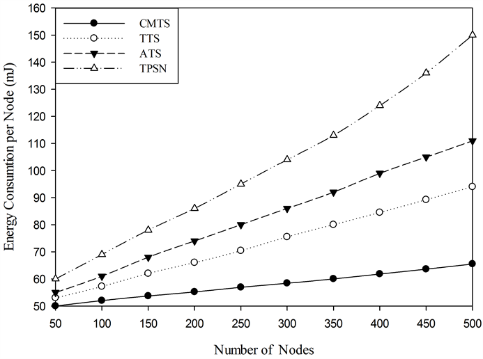 Figure 5. Effect of number of nodes on energy consumption in CMTS, TTS, ATS and TPSN.

Figure 6. Effect of hops over synchronization error in CMTS, ATS, TSS and TPSN.
5. Conclusion
Time synchronization in wireless sensor networks is challenging problem due to high delay variability and resource constraints of nodes. In critical applications, time synchronization is very important to know the exact time of the event. This paper proposes a mobile node based time synchronization algorithms named CMTS for wireless sensor networks. In CMTS, mobile nodes move on a fixed path with certain velocity. Synchronization process is initiated by mobile node and it synchronizes sensor nodes falling in its communication range. The objective of mobile nodes is to reduce the communication overhead for sensor nodes and to do synchronization with higher precision. Simulation results show that the proposed algorithm is able to save the energy, reduce synchronization time and improve synchronization accuracy.
Cite this paper
Gautam, G.C. and Kaushal, N.C. (2017) Controlled Mobility Time Synchronization for WSNs. Wireless Sensor Network, 9, 1-15. http://dx.doi.org/10.4236/wsn.2017.91001
References
- 1. Schmid, T., Charbiwala, Z., Friedman, J., Cho, Y.H. and Srivastava, M.B. (2008) Exploiting Manufacturing Variations for Compensating Environment Induced Clock Drift in Time Synchronization. ACM SIGMETRICS Performance Evaluation Review—SIGMETRICS’08, 36, 97-108.
https://doi.org/10.1145/1384529.1375469 - 2. Li, Q. and Rus, D. (2006) Global Clock Synchronization in Sensor Networks. IEEE Transactions on Computers, 55, 214-226.
https://doi.org/10.1109/TC.2006.25 - 3. Li, L., Liu, Y., Yang, H. and Wang, H. (2008) A Precision Adaptive Average Time Synchronization Protocol in Wireless Sensor Networks. Proceedings of the IEEE International Conference on Information and Automation, Zhangjiajie, 20-23 June 2008.
https://doi.org/10.1109/icinfa.2008.4607969 - 4. Elson, J., Girod, L. and Estrin, D. (2002) Fine-Grained Network Time Synchronization Using Reference Broadcasts. Proceedings of the 5th Symposium on Operating Systems Design and Implementation, Boston, 9-11 December 2002, 147-163.
https://doi.org/10.1145/1060289.1060304 - 5. Hong, Y.-W. and Scaglione, A. (2005) A Scalable Synchronization Protocol for Large Scale Sensor Networks and Its Applications. IEEE Journal on Selected Areas in Communications, 23, 1085-1099.
https://doi.org/10.1109/JSAC.2005.845418 - 6. Zhou, D. and Lai, T.-H. (2007) An Accurate and Scalable Clock Synchronization Protocol for IEEE 802.11-Based Multi Hop Ad Hoc Networks. IEEE Transactions on Parallel and Distributed Systems, 18, 1797-1808.
https://doi.org/10.1109/TPDS.2007.1116 - 7. Mills, D.L. (1991) Internet Time Synchronization: The Network Time Protocol. IEEE Transactions on Communication, 39, 1482-1493.
https://doi.org/10.1109/26.103043 - 8. Ganeriwal, S., Kumar, R. and Srivastava, M.B. (2003) Timing-Sync Protocol for Sensor Networks. Proceedings of the 1st International Conference on Embedded Networked Sensor Systems, Los Angeles, 5-7 November 2003, 138-149.
https://doi.org/10.1145/958491.958508 - 9. Van Greunen, J. and Rabaey, J. (2003) Lightweight Time Synchronization for Sensor Networks. Proceedings of the 2nd ACM International Conference on Wireless Sensor Networks and Applications (WSNA’03), San Diego, 19 September 2003, 11-19.
https://doi.org/10.1145/941350.941353 - 10. Maroti, M., Kusy, B., Simon, G. and Lédeczi, á. (2004) The Flooding Time Synchronization Protocol. Proceedings of the 2nd International Conference on Embedded Networked Sensor Systems, Baltimore, 3-5 November 2004, 39-49.
https://doi.org/10.1145/1031495.1031501 - 11. Dai, H. and Han, R. (2004) Tsync: A Lightweight Bidirectional Time Synchronization Service for Wireless Sensor Networks. ACM SIGMOBILE Mobile Computing and Communications Review, 8, 125-139.
https://doi.org/10.1145/980159.980173 - 12. Sichitiu, M.L. and Veerarittiphan, C. (2003) Simple, Accurate Time Synchronization for Wireless Sensor Networks. IEEE Conference on Wireless Communications and Networking (WCNC), New Orleans, 16-20 March 2003, 1266-1273.
https://doi.org/10.1109/wcnc.2003.1200555 - 13. Noh, K.-L., Serpedin, E. and Qaraqe, K.A. (2008) A New Approach for Time Synchronization in Wireless Sensor Networks: Pairwise Broadcast Synchronization. IEEE Transactions on Wireless Communications, 7, 3318-3322.
https://doi.org/10.1109/TWC.2008.070343 - 14. Ren, F., Lin, C. and Liu, F. (2008) Self-Correcting Time Synchronization Using Reference Broadcast in Wireless Sensor Network. IEEE Wireless Communications, 15, 79-85.
https://doi.org/10.1109/MWC.2008.4599225 - 15. Liu, B., Ren, F., Shen, J. and Chen, H. (2010) Advanced Self-Correcting Time Synchronization in Wireless Sensor Networks. IEEE Communications Letters, 14, 309-311.
https://doi.org/10.1109/LCOMM.2010.04.092364 - 16. Pussente, R.M. and Barbosa, V.C. (2009) An Algorithm for Clock Synchronization with the Gradient Property in Sensor Networks. Journal of Parallel and Distributed Computing, 69, 261-265.
https://doi.org/10.1016/j.jpdc.2008.11.001 - 17. Simeone, O., Spagnolini, U., Scutari, G. and Bar-Ness, Y. (2008) Physical-Layer Distributed Synchronization in Wireless Networks and Applications. Physical Communication, 1, 67-83.
https://doi.org/10.1016/j.phycom.2008.01.003 - 18. Song, H., Zhu, S. and Cao, G. (2007) Attack-Resilient Time Synchronization for Wireless Sensor Networks. Ad Hoc Networks, 5, 112-125.
https://doi.org/10.1016/j.adhoc.2006.05.016 - 19. Hoepman, J.-H., Larsson, A., Schiller, E.M. and Tsigas, P. (2011) Secure and Self-Stabilizing Clock Synchronization in Sensor Networks. Theoretical Computer Science, 412, 5631-5647.
https://doi.org/10.1016/j.tcs.2010.04.012 - 20. Liu, J. (2008) Scalable Synchronization of Clocks in Wireless Sensor Networks. Ad Hoc Networks, 6, 791-804.
https://doi.org/10.1016/j.adhoc.2007.07.001 - 21. Olfati-Saber, R. and Murray, R.M. (2004) Consensus Problems in Networks of Agents with Switching Topology and Time-Delays. IEEE Transactions on Automatic Control, 49, 1520-1533.
https://doi.org/10.1109/TAC.2004.834113 - 22. Rentel, C.H. and Kunz, T. (2008) A Mutual Network Synchronization Method for Wireless Ad Hoc and Sensor Networks. IEEE Transactions on Mobile Computing, 7, 633-646.
https://doi.org/10.1109/TMC.2007.70787 - 23. Chen, J., Yu, Q., Zhang, Y., Chen, H.-H. and Sun, Y. (2010) Feedback Based Clock Synchronization in Wireless Sensor Networks: A Control Theoretic Approach. IEEE Transactions on Vehicular Technology, 59, 2963-2973.
https://doi.org/10.1109/TVT.2010.2049869 - 24. Cooklev, T., Eidson, J.C. and Pakdaman, A. (2007) An Implementation of IEEE 1588 over IEEE 802.11b for Synchronization of Wireless Local Area Network Nodes. IEEE Transactions on Instrumentation and Measurement, 56, 1632-1639.
https://doi.org/10.1109/TIM.2007.903640 - 25. Noh, K.-L., Chaudhari, Q.M., Serpedin, E. and Suter, B.W. (2007) Novel Clock Phase Offset and Skew Estimation Using Two-Way Timing Message Exchanges for Wireless Sensor Networks. IEEE Transaction on Communications, 55, 766-777.
https://doi.org/10.1109/TCOMM.2007.894102 - 26. Sari, I., Serpedin, E., Noh, K.-L., Chaudhari, Q. and Suter, B. (2008) On the Joint Synchronization of Clock Offset and Skew in RBS-Protocol. IEEE Transaction on Communications, 56, 700-703.
https://doi.org/10.1109/TCOMM.2008.060184 - 27. Wang, J., Zhang, S., Gao, D. and Wang, Y. (2014) Two-Hop Time Synchronization Protocol for Sensor Networks. EURASIP Journal on Wireless Communications and Networking, 2014, 39.
https://doi.org/10.1186/1687-1499-2014-39 - 28. Djenouri, D., Merabtine, N., Mekahlia, F.Z. and Doudou, M. (2013) Fast Distributed Multi-Hop Relative Time Synchronization Protocol and Estimators for Wireless Sensor Networks. Ad Hoc Networks, 11, 2329-2344.
https://doi.org/10.1016/j.adhoc.2013.06.001 - 29. Wu, J., Jiao, L. and Ding, R. (2012) Average Time Synchronization in Wireless Sensor Networks by Pair Wise Messages. Computer Communications, 35, 221-233.
https://doi.org/10.1016/j.comcom.2011.09.007 - 30. Schmid, T., Charbiwala, Z., Shea, R. and Mani, S.B. (2009) Temperature Compensated Time Synchronization. IEEE Embedded Systems Letters, 1, 37-41.
https://doi.org/10.1109/LES.2009.2028103 - 31. Huang, G., Zomaya, A.Y., Delicato, F.C. and Pires, P.F. (2014) Long Term and Large Scale Time Synchronization in Wireless Sensor Networks. Computer Communications, 37, 77-91.
https://doi.org/10.1016/j.comcom.2013.10.003 - 32. Dantu, K., Rahimi, M., Shah, H., Babel, S., Dhariwal, A. and Sukhatme, G.S. (2005) Robomote: Enabling Mobility in Sensor Networks. The 4th International Symposium on Information Processing in Sensor Networks, 15 April 2005, 404-409.
https://doi.org/10.1109/ipsn.2005.1440957 - 33. Friedman, J., Lee, D.C., Tsigkogiannis, I., Wong, S., Chao, D., Levin, D., Kaisera, W.J. and Srivastava, M.B. (2005) RAGOBOT: A New Platform for Wireless Mobile Sensor Networks. In: Prasanna, V.K., Iyengar, S.S., Spirakis, P.G. and Welsh, M., Eds., Distributed Computing in Sensor Systems, Springer, Berlin Heidelberg, 412.
https://doi.org/10.1007/11502593_43 - 34. Bergbreiter, S. and Pister, K.S.J. (2003) CotsBots: An Off-the-Shelf Platform for Distributed Robotics. Proceedings of the IEEE/RSJ International Conference on Intelligent Robots and Systems (IROS 2003), 27-31 October 2003, 1632-1637.
https://doi.org/10.1109/iros.2003.1248878