Wireless Sensor Network
Vol.07 No.06(2015), Article ID:57535,32 pages
10.4236/wsn.2015.76006
A Novel Low-Complexity Low-Latency Power Efficient Collision Detection Algorithm for Wireless Sensor Networks
Fawaz Alassery, Walid K. M. Ahmed, Mohsen Sarraf, Victor Lawrence
Electrical and Computer Engineering Department, Stevens Institute of Technology, Hoboken, NJ, USA
Email: falasser@stevens.edu
Copyright © 2015 by authors and Scientific Research Publishing Inc.
This work is licensed under the Creative Commons Attribution International License (CC BY).
http://creativecommons.org/licenses/by/4.0/


Received 1 May 2015; accepted 26 June 2015; published 29 June 2015
ABSTRACT
Collision detection mechanisms in Wireless Sensor Networks (WSNs) have largely been revolving around direct demodulation and decoding of received packets and deciding on a collision based on some form of a frame error detection mechanism, such as a CRC check. The obvious drawback of full detection of a received packet is the need to expend a significant amount of energy and processing complexity in order to fully decode a packet, only to discover the packet is illegible due to a collision. In this paper, we propose a suite of novel, yet simple and power-efficient algorithms to detect a collision without the need for full-decoding of the received packet. Our novel algorithms aim at detecting collision through fast examination of the signal statistics of a short snippet of the received packet via a relatively small number of computations over a small number of received IQ samples. Hence, the proposed algorithms operate directly at the output of the receiver's analog-to-digital converter and eliminate the need to pass the signal through the entire. In addition, we present a complexity and power-saving comparison between our novel algorithms and conventional full-decoding (for select coding schemes) to demonstrate the significant power and complexity saving advantage of our algorithms.
Keywords:
Wireless Sensor Networks, Wireless Sensor Protocols, Collision Detection Algorithms, Power-Efficient Techniques, Low Complexity Algorithms

1. Introduction
Most research activities in WSNs focus on maximizing the network lifetime and minimizing the power consumption since they are powered by using finite energy sources (e.g., batteries). In this regard, some efforts deal with the routing schemes in order to rout a packet through most energy efficient links from a source node to a destination ([1] -[3] ), while other researches extensively explore MAC schemes ([4] -[6] ) which efficiently reduce packets collisions. However, MAC layer schemes intrinsically cannot eliminate all kind of collisions, because of hidden nodes problems, as well as collisions when multiple nodes sense the medium free at the same time followed by transmitting their packets. Hence the collision may occur at the receiver where it is difficult to distinguish between desirable and interferers signals.
Authors in [7] , investigate the effect of interference signals on decoding power. They suggest adapting the decoder power based on the communication range. That is the decoder power needed to be increased, while transmitter power needs to be decreased for short rang communication systems. Authors in [8] , design LDPC decoder architecture for low power WSNs. They suggest different LDPC codes and analyze the energy saving for encoded communication system. Their analysis shows how the decoder power levels affect the Bit Error Rate (BER). Author in [9] , investigate the trade-off between the transmission power and decoding power in WSNs by employing convolutional codes with a specific ECC complexity in order to extend the network lifetime. In [10] , the authors studied the relationship between the number of received bits and the decoder power consumption using LDPC codes in WSNs. Their analysis shows a large improvement in the network lifetime up to four times with LDPC codes which is more efficient than the convolutional and block codes. A power management technique at the receiver side in WSNs has been presented in [11] . Authors used rateless codes to minimize the power consumption, and their analytical results showed up to 80% of energy that is saved in comparison with IEEE 802.15.4 physical layer standard. Some efforts (e.g. [12] ) focused on the actual design of LDPC decoder where early stopping methods are proposed in order to reduce the number of unnecessary iterations when decoding received packets. Such method is efficient in low SNR but it has a limitation when SNR is high.
Error correction schemes in wireless communication systems increase the reliability between a transmitter and receiver by reducing the probability of error. Reducing the probability of error can be achieved by increasing the transmit power or using a complex decoder that consume too much power to decode every received packet correctly. However, in limited power recourses networks such as WSNs, such increase in the transmit power as well as decoding power are not efficient since it contradicts with the design objective of WSNs which aims at energy-efficient solutions. Hence, in WSNs a fundamental trade-off exists between the transmitter and receiver power that should be considered to enhance the network lifetime.
One of the main sources of overhead power consumption in WSNs is collision detection. When multiple sensors transmit at the same time, their transmitted packets collide at the central node (the receiver) [13] . Authors in [14] use out of band control channel to indicate the transmission status (i.e. active state) for sensors which have packets ready to be transmitted. Sensors sense the control channel to detect collision. However, such technique is not accurate to detect collisions that may occur at the receiver. In addition, current collision detection mechanisms have largely been revolving around direct demodulation and decoding of received packets and deciding on a collision based on some form of a frame error detection mechanism, such as a CRC check [15] . The obvious drawback of full decoding of a received packet is the need to expend a significant amount of energy and processing complexity in order to fully-decode a packet, only to discover the packet is invalid and corrupted due to collision. So, decoding of corrupted packets becomes useless and provides the main cause of unnecessary power consumption.
In this paper we pose the following questions: Can we propose a power-efficient technique to detect packets’ collisions at the receiver side of WSNs without the need for full-decoding of received packets? Further, can we eliminate the need to pass corrupted packets through the entire demodulator/decoder? From the perspective of achieving an efficient collision detection scheme at the receiver-side of WSNs we propose a suite of novel, yet simple and power-efficient algorithms to detect a collision without the need for full-decoding of the received packet. Our novel approach aims at detecting collision through fast examination of the signal statistics of a short snippet of the received packet via a relatively small number of computations over a small number of received IQ samples. Hence, operating directly at the output of the receiver’s analog-to-digital-converter (ADC) and eliminating the need to pass the signal through the entire demodulator/decoder line-up. Figure 1 illustrates where we apply our proposed scheme. In addition, we present a complexity and power-saving comparison between our novel Statistical Discrimination (SD) algorithms and conventional Full-Decoding (FD) algorithm (i.e. Soft Output Viterbi Algorithm) to demonstrate the significant power and complexity saving advantage of our scheme. Accordingly, our novel SD scheme has the following advantages:
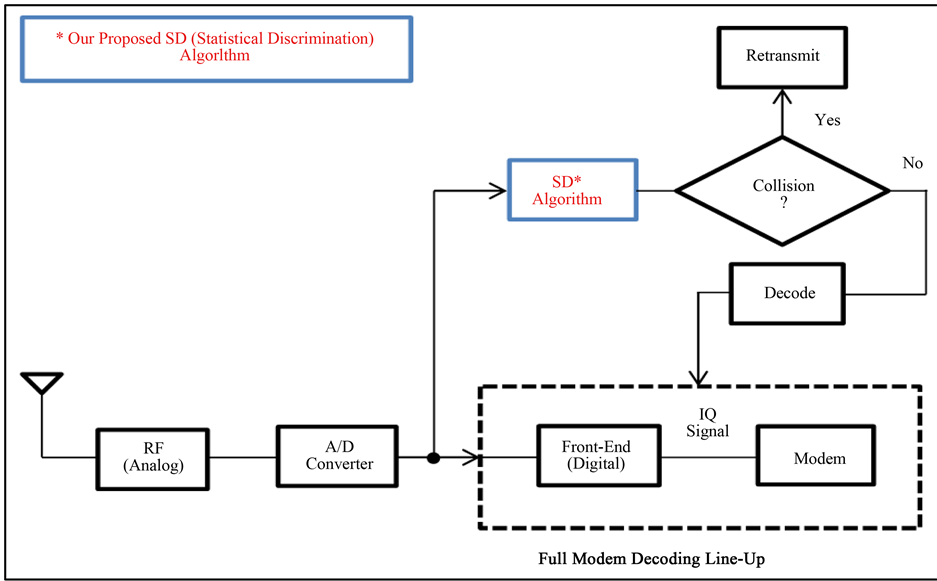
Figure 1. Block diagram for a receiver’s line-up.
・ The SD scheme not only reduces processing complexity and hence power consumption, but it also reduces the latency incurred to detect a collision since it operates on only a small number of samples-that may be chosen to be in the beginning of a received packet-instead of having to buffer and process the entire packet as is the case with a Full-Decoding (FD) algorithms.
・ The SD scheme does not require any special pilot or training patterns. It operates directly on the (random) data, i.e., the received packet as is.
・ With a relatively short measurement period, the SD scheme can achieve low False-Alarm and Miss probabilities. It achieves a reliable collision-detection mechanism at the receiver-side of WSNs in order to minimize the receiption power consumption.
・ The SD scheme can be turned over various design parameters in order to allow a system designer multiple degrees of freedom for design trade-offs and optimization.
The remainder of this paper is organized as follows. Section 2 describes our system. In section 3, we explain the proposed algorithms and show how to select a system threshold level. In section 4, we evaluate the power saving based on our proposed algorithms. In addition, we compare the computational complexity of our algorithms against commonly used decoding techniques (e.g., Soft Output Viterbi Algorithm, or SOVA). In section 5, we provide analysis and numerical empirical characterization to provide some quantitative theoretical framework and shed some light on the behavior of the various system factors and parameters involved in our proposed algorithms. In section 6, we present performance results, and finally in section 7 we provide the conclusion for this paper.
2. System Description
Figure 2 depicts an example of a WSN where a number of intermediate sensors are deployed arbitrarily to perform certain functionalities including sensing and/or collecting data and then communicating such information to a central sensor node (a receiver). The central node may process and relay the aggregate information to a backbone network.
As seen in Figure 2, there are N wireless sensors that communicate to the central node, where at any point in time, multiple packets may accidentally arrive simultaneously and cause a collision. Without loss of generality, we shall assume for the sake of argument that one sensor is denoted a “desirable” sensor, while the rest of the
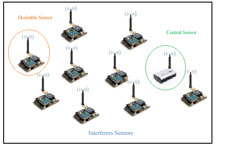
Figure 2. Wireless Sensor Network (WSN) with one desirable sensor, multiple interferer sensors and a central sensor (a receiver).
colliding sensors become “interferers”. We assume the maximum number of sensors i.e., N = 30. This number can be tuned as required is order to meet designers’ requirements.
A commonly accepted model for packet arrivals, i.e., a packet is available at a sensor and ready to be transmitted, is the well-known Bernoulli-trial-based arrival model, where at any point in time, the probability that a sensor has a packet ready to transmit is α.
Upon the receipt of a packet, the central node processes and evaluates the received packet and makes a decision on whether the packet is a collision-free (good) or has suffered a collision (bad). In this paper, we propose a suite of fast collision detection algorithms where the central node evaluates the statistics of the received signal’s IQ samples at the output of the receiver’s ADC directly using a simple SD scheme (as will be explained in more detail in the following sections), saving the need to expend power and time on the complex modem line-up processing (e.g., demodulation and decoding). If the packet passes the SD test, it is deemed collision-free and undergoes all the necessary modem processing to demodulate and decode the data. Otherwise, the packet is deemed to have suffered a collision, which in turn triggers the central node to issue a NACK message per the mechanism and rules mandated by the specific multiple-access scheme employed in the network.
It is noted that the actual design details and choice of the multiple access mechanism, e.g., slotted or un-slot- ted Aloha, are beyond the scope of this paper and irrelevant to the specifics of the technique proposed herein.
3. Algorithm Description
As mentioned earlier, our proposed algorithms are based upon evaluating the statistics of the received signal at the receiver ADC output via the use of a simple statistical discrimination metrics calculation that are performed on a relatively small portion of the received IQ packet samples. The resulting metrics values are then compared with a pre-specified threshold level to determine if the statistics of the samples of received signals reflect an acceptable signal-to-interference-plus-noise ratio (SINR) from the decoding mechanism perspective. If so, the packed is deemed collision-free and qualifies for further decoding. Otherwise, the packet is deemed to have suffered a collision with other interferer(s) and is rejected without expending any further processing/decoding energy. A repeat request may then be issued so the transmitting sensors to re-try depending on the MAC scheme. In other words, the idea is to use a fast and simple calculation to determine if the received signal strength (RSS) is indeed due to a single transmitting sensor that is strong enough to achieve an acceptable SINR at the central node’s receiver, or the RSS is rather due to the superposition of the powers of multiple colliding packets, hence the associated SINR is less than acceptable to the decoding mechanism.
Let’s define the kth received signal (complex-valued) IQ sample at the access node as:

where ,
,  ,
,

Is a complex-valued quantity that represents the kth IQ sample component contributed by the desired sensor, and

Is the kth IQ sample component contributed by the mth interfering (colliding) sensor? Finally, 
Is a complex-valued Additive-White-Gaussian Noise (AWGN) quantity (e.g., thermal noise).
We propose three time-averaging statistical discrimination (SD) metrics that are applied to the envelope value, , of the received IQ samples at the central node as follows:
1) Entropy (Logarithmic) based metric:
 (1)
(1)
2) Moment based metric1:
 (2)
(2)
3) Signal Dynamic-Range Maximum-Minimum based metric:
 (3)
(3)
The computed statistical discrimination metric is then compared with a pre-specified threshold value that is set based on a desired signal-to-interference-plus-noise ratio (SINR) cut-off assumption2, . That is (and as will be described in more detail later in this paper), a system designer pre-evaluates the appropriate threshold value that corresponds to the desired
 . If the SD metric value is higher than the threshold value, then the SD metric value reflects a SINR that is less than
  and the packet is deemed not usable, and vice-versa. Accordingly, a “False-Alarm” event occurs if the received SINR is higher than
  but the SD algorithm erroneously deems the received SINR to be less than
 . On the other hand, if the SD algorithm deems the SINR to be higher than
  while it is actually less than
 , a “Miss” event is encountered. Miss and False-Alarm probabilities directly impact the overall system performance as will be discussed in the following sections. Therefore, it is desired to minimize such probabilities as much as possible.
Threshold Selection
The decision threshold is chosen based on evaluating the False-Alarm and Miss probabilities and choosing the threshold values that satisfy the designer’s requirements of such quantities. For example, we generate, say, a 100,000 Monte-Carlo simulated snapshots of interfering sensors (e.g., 1 - 30 sensors with random received powers to simulate various path loss amounts) where for each snapshot we compute the statistical discrimination value for the received SINR and compare it with various threshold levels, determine if there is a corresponding False-Alarm or Miss event and record the counts of such events. At the end of the simulations the False-Alarm and Miss probabilities are computed and plotted versus the range of evaluated threshold values, which in-turn, enables the designer to determine a satisfactory set point for the threshold.
4. Power Saving Analysis
To analyze the power saving of our proposed SD system we introduce the following computational complexity metrics:
 (4)
(4)
 (5)
(5)
In above formulas, S is the number of computational operations incurred in our proposed scheme, while F is the number of computational operations incurred in a full-decoding scheme,  and
and  are the probabilities of Miss and False-Alarm events respectively. Hence,
  represents the computational complexity for the case where the central node (the receiver) makes a wrong decision to fully-decode the received packet (i.e., declared as a collision-free packets) while the packet should has been rejected (i.e., due to collision). On the other hand,
  is the computational complexity for the case where the central node makes a correct decision to fully decode received packet.
In addition, and for the comparison purposes, we introduce the following formulae in order to compare the computational complexity saving achieved by our proposed SD approach (i.e., ) over the FD approach (i.e.,
 ):
):
 (6)
(6)
 (7)
(7)
In above formulae,  and
and  are the probabilities of collision and no-collision events respectively.
  and
and  have been obtained via Monte-Carlo simulation as follows: A random number of interfering sensors (maximum of 30 sensors) is generated per a simulation snapshot, where each sensor is assumed to have a randomly received power level at the access node (to reflect a random path loss/location effect). The generation of the interfering sensors is based on a Bernoulli trial model where it is assume that the probability of a packet available for transmission at a sensor (hence the existence/generation of the sensor for the snapshot at hand) is equal to
 . If the total SINR is found to be worse than the cut-off limit, a collision is assumed and vice-versa. For our numerical example in this section we used
  and
and . Also, we typically generate more than 100,000 snapshots in order to achieve a reliable estimate of the collision probabilities. For the aforementioned choices of
  and
and , we found the collision probabilities to be
  and
and .
.
Comparing with Full-Decoding Algorithms
In order to assess the computational complexity of our SD scheme, we first quantize our metrics calculation in order to define fixed-point and bit-manipulation requirement of such calculations. We also assume a look-up table (LUT) approach for the logarithm calculation. Note that the number of times the algorithm needs to access the LUT equals the number of IQ samples involved in the metric calculation. Thus, our algorithm only needs to perform addition operations as many times as the number of samples. Hence, if the number of bits per LUT word/entry is equal to M at the output of the LUT, our algorithm needs as many M-bit addition operations as the number of IQ samples involved in the metric calculation.
As a case-study, we compare the complexity of our SD scheme with the complexity of a FD algorithm assuming a Soft Output Viterbi Algorithm (SOVA). SOVA has been an attractive choice for WSNs [16] . Authors in [17] measure the computational complexity of SOVA (per information bit of the decoded codeword) based on the size of the encoder memory. It has been shown in [17] that for a memory length of , the total computational complexity per information bit can be estimated as:
 (8)
(8)
In contrast, our SD system does not incur such complexity related to the size of the encoder memory. In addition, our SD system avoids other complexities required by a full decoding such as time and frequency synchronization, Doppler shift correction, fading and channel estimation, etc., since our SD scheme operates directly at the IQ samples at the output of the ADC “as is”. Finally, the FD approach requires buffering and processing of the entire packet/codeword while our SD scheme needs only to operate on a short portion of the received packet.
Now let’s compute the computational complexity for our SD approach using the logarithmic (entropy) metric. Let’s assume that the IQ ADCs each is D bits. Also, let’s assume a  operation is done through a LUT approach to save multiplication operations. In addition, let’s also assume that the square-root,
  , is also done through a LUT approach. Hence, each of the
  and
and  operations consume of the order of D bit-comparison operations to address the
  LUT. Then, if the output of the LUT is G bits, it follows that we need about G bit additions for an
  operation. Let’s assume that the
  LUT has G bits for input addressing and K output bits. Then, we need about G+1 bit-comparison operations to address the
  LUT. Let’s assume a
 is also done through a K-bit-input/L-bit-output LUT. Hence, a
  costs about K bit-com-
parison operations to address the  LUT. Finally, for simplicity, let’s assume that a bit comparison operation costs as much as a bit addition operation3. Accordingly, the total number of operations needed to compute the
  for one IQ sample is:
 (9)
(9)
If we assume the IQ over-sampling rate (OSR) to be Z (i.e., we have Z samples per information symbol), then we need about  bit additions to add the
  values for every information symbol. Hence, for one information symbol, we need a total of:
 (10)
(10)
Now if we assume an M-ary modulation (i.e.,  information bits are mapped to one symbol), then the computational complexity per information bit can be computed as:
 (11)
(11)
For example, in order to show the complexity saving of our SD algorithm, let’s assume a QPSK modulation scheme (M = 4). Also, let’s assume Z = 2 (2 samples per symbol), and D = G = K = L = 10 bits, which represents a good bit resolution. Also, let’s assume a memory size of  for the SOVA decoder. Using the formulae (8), it follows the SOVA FD algorithm costs 271 operations per an information bit while our Entropy (Logarithmic) SD algorithm based on formula (11) costs only 61 operations per an information bit, which represents a 77% saving on the computational complexity.
In addition, in a no-collision event, the SD algorithm check would represent a processing overhead. Nonetheless, our SD scheme still provides a significant complexity saving over the FD scheme as demonstrated by the following example. Table 1 in Appendix A shows the probability of Miss and False-Alarm to be 0.0762 and 0.0684, respectively for QPSK and a 50 bits measurement period4. Now, based on formulae (4) and (5),  and
and  (per information bit) for our SD algorithm will equal:


For the comparison purposes between our SD algorithm and SOVA FD algorithm, formulae (6) and (7) are used to find the computational complexity when no-collision is detected:


Hence, the complexity savings (in number of operations per information bit) becomes:

Note that the above complexity saving calculation, in fact, represents a lower bound on the saving since the above calculation did not take into account the modem line-up operational complexity in order to demodulate and receive the bits in their final binary format properly (i.e., synchronization, channels estimation, etc.).
The performance of our algorithms can be tuned as desired by a system designer. Appendix A provides performance comparisons for various examples where the system designer may choose to reduce the measurement period (e.g., to 25 or 50 bits) at the expense of increasing the Miss and False-Alarm probabilities, or may increase the throughput by using a longer estimation period in order to improve the accuracy of the statistical discriminator performance and reduce the Miss and False-Alarm probabilities (i.e. our system throughput  is defined as
 ; Where
  denotes the False-Alarm probability).
5. Empirical Characterization
In this section, we attempt at empirically characterizing the statistics of various key quantities considered and encountered in this work, in an attempt to shed some light onto the behavior of such quantities and pave the way for some analytic mathematical tractability.
5.1. Statistics of the IQ Signal Envelope
In order to obtain reliable statistics, we have simulated different scenarios that reflect reasonably realistic assumptions5. For example, in our simulations, we assume that packets are generated at the various sensors using a Bernoulli trial model. That is, the probability of a packet available for transmission at a sensor is equal to α. We also generate random number of sensors per a network snapshot that are placed at random locations and distances from the central node in order to reflect various/random path loss situations6. The individual received sensor and noise components at the access node, as well as the total received signal (the superposition of the sensor received signals plus AWGN) are always normalized properly to reflect the correct SINR assumption.
In general, the parameters covered in this investigation include:
・ Number of sensors7.
・  level. For our simulations, we typically assumed
  8.
8.
・ Sensitivity (tolerance) around the . That is, if the received SINR is within, for example, 1 dB, 1.5 dB, -2 dB, -10 dB or etc. around
  (5 dB), we denote such SINR tolerance level as
 .
.
・ Probability of transmission per sensor.
・ Modulation scheme.
・ Measurement duration.
・ SD metric choice.
As seen from the above simulation setting list, the simulations are always run assuming a fixed SINR value, in order to enforce a collision, or a no-collision event for the entire simulation session. Accordingly, the statistical analysis and characterization in this section are evaluated conditional on a collision or no-collision event in order to isolate the statistical characteristics of the metrics from the collision statistics, which can be dependent upon the MAC mechanism and other system parameters such as the specifics of the path loss distributions encountered by the sensors, which would affect the level of the received SINR …etc.
In general, we have found that the Normal (Gaussian) distribution has the closest fit to the actual (simulated) PDF of received signal envelope when SINR ≥ 0 dB. For SINR < 0 dB, however, the Rayleigh distribution seems to be a better fit. We qualify the fitting accuracy of a distribution using the least-mean-square error (LMSE) criterion. Accordingly, the Normal and Rayleigh distributions have exhibited the minimum LMSE in comparison with other distributions as seen in Figure 3 and Figure 4 (such as 5th degree polynomial fit, the Weibull
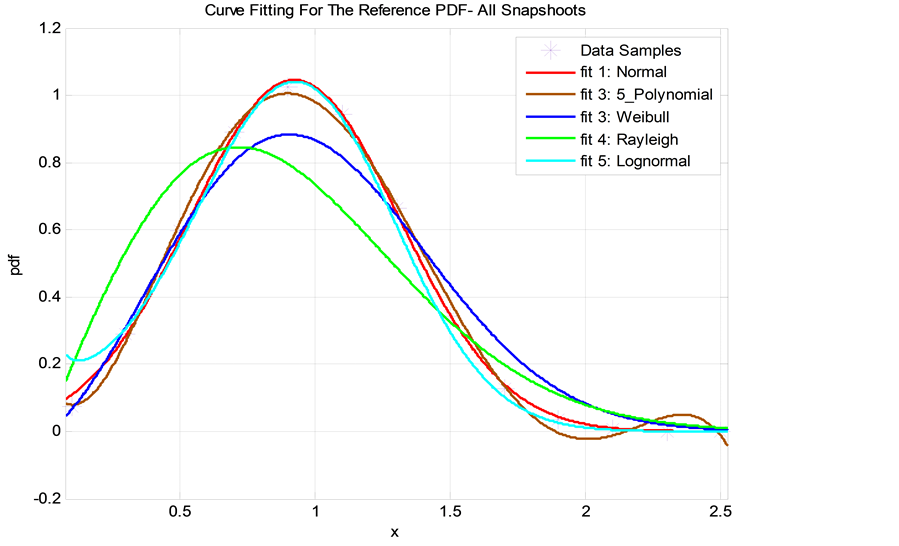
Figure 3. A curve-fitting comparison of various statistical distributions overlaid on the actual PDF for the IQ signal envelope as obtained from Monte-Carlo simulations: Logarithmic metric, SINR = 4 dB.
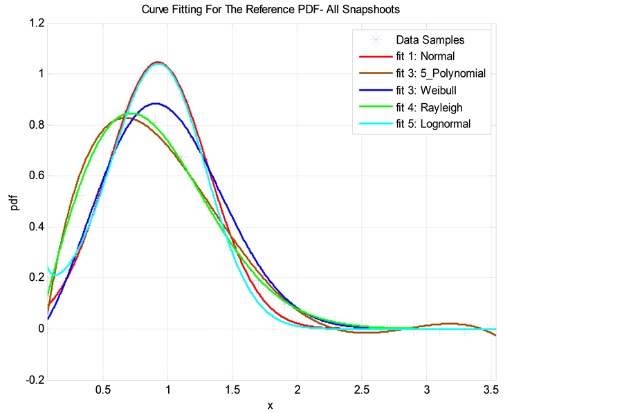
Figure 4. A curve-fitting comparison of various statistical distributions overlaid on the actual PDF for the IQ signal envelope as obtained from Monte-Carlo simulation: Logarithmic metric, SINR = −6 dB.
distribution and the Log-normal distribution).
For example, in Figure 3, the normal distribution with mean , variance
  resulted in a LMSE = 0.0024 and exhibited the closest fit to the actual (simulated) PDF of the received signal envelope. The choice of parameters for this example has been as follows:
・ Maximum number of sensors is 30 (i.e., the number of simultaneous sensors existing in the network per a simulation snapshot is between 2 and 30 sensors).
・  , SINR = 4 dB
 .
.
・ Probability of a packet available for transmission at a sensor is 0.3 (i.e., theBernoullitrial model probability is ).
).
・ Modulation scheme is 8PSK.
・ Measurement period is equal to 50 information bits.
・ Logarithmic (entropy) metric.
In Figure 4, the Rayleigh distribution achieved a LMSE = 0.0032 and exhibited the closest fit to the PDF of received signal envelop. Again, the choice of parameters in this figure is assumed as follows:
・ Maximum number of sensors is 30.
・  , SINR = -6 dB
 .
.
・  .
.
・ Modulation scheme is 8 PSK.
・ Measurement period is equal to 50 information bits.
・ Logarithmic (entropy) metric.
Figure 5 and Figure 6 show similar examples for a 3rd moment SD metric. Figure 5 shows how the Normal distribution continues to have the closest fit and achieves a LMSE = 0.0036, while in Figure 6 the Rayleigh distribution has the best fit with LMSE = 0.0041. The choice of parameters follows:

Figure 5. A curve-fitting comparison of various statistical distributions overlaid on the actual PDF for the IQ signal envelope as obtained from Monte-Carlo simulations: 3rd moment metric, SINR = 3 dB.
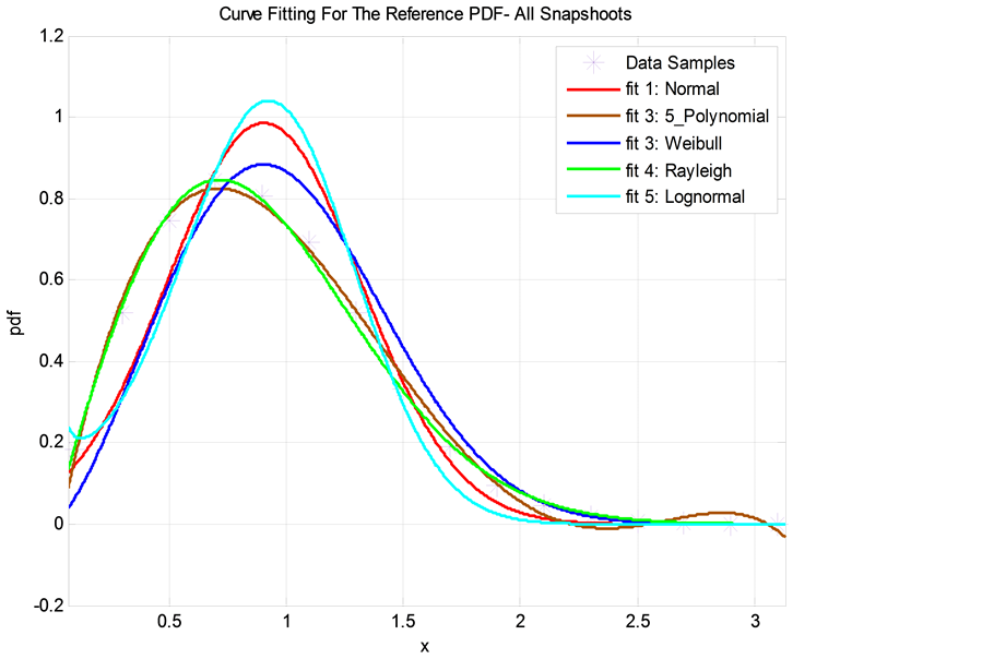
Figure 6. A curve-fitting comparison of various statistical distributions overlaid on the actual PDF for the IQ signal envelope as obtained from Monte-Carlo simulation: 3rd moment metric, SINR = −4 dB.
・ Maximum number of sensors is 30.
・  , SINR = 3 dB
  for Figure 5, while
 , SINR = -4 dB
  for Figure 6.
・  .
.
・ Modulation scheme is QPSK.
・ Measurement period is 200 information bits.
・ 3rd moment metric.
Figure 7 and Figure 8 show corresponding examples for the MAX-MIN based metric. Again, the Normal and Rayleigh distributions have best fits with LMSE = 0.0039 and LMSE = 0.0220, respectively. Our choice of parameters follows:
・ Maximum number of sensors is 30.
・  , SINR= 3 dB
  for Figure 7, while
 , SINR = -5 dB
  for Figure 8.
・  .
.
・ Modulation scheme is 16 PSK.
・ Measurement period is 1000 information bits.
MAX-MIN based metric.
5.2. Statistics of the SD Metrics
In general, the ensemble (overall) average (mean) of the first moment of the IQ envelope of the received signal, as well as the second moment (i.e., the power of received signal) is a function of the received SINR. In the following, we plot the ensemble averages of the first and second moments (in Figure 9 and Figure 10 respectively) of the IQ envelope quantity viruses the corresponding first and second moment values that correspond to the best fitting distribution (i.e., Normal and Rayleigh PDFs as pointed out above). The parameters in Figure 9 and

Figure 7. A curve-fitting comparison of various statistical distributions overlaid on the actual PDF for the IQ signal envelope as obtained from Monte-Carlo simulations: MAX- MIN based metric, SINR = 3 dB.

Figure 8. A curve-fitting comparison of various statistical distributions overlaid on the actual PDF for the IQ signal envelope as obtained from Monte-Carlo simulations: MAX- MIN based metric, SINR = −5 dB.

Figure 9. The mean μ for the received signal envelope for the simulation data samples & curve fitting distribution vs. SINR.

Figure 10. The second moment for the received signal power for the simulation data samples & curve fitting distribution vs. SINR.
Figure 10 are assumed as follows:
・ Maximum number of sensors is 30.
・  , SINR = [-8 dB, 8 dB], i.e., the interval between -8 dB and 8 dB.
・  .
.
・ Modulation scheme is 8 PSK.
・ Measurement period is 200 information bits.
Logarithmic metric.
In addition, we have found that the normal distribution has the best fit to the simulated PDFs for the Logarithmic, Moment and MAX-MIN based metrics9. The corresponding normal curve fittings are shown in Figures 11-13 for logarithmic, moment and MAX-MIN based metrics respectively.
Based on the normal PDF fit [19] , one can calculate the False-Alarm and Miss probabilities as follows: If we assume a pre-defined threshold level , then it can be shown that:
 (12)
(12)
 (13)
(13)
It should be noted that direction of the metric threshold-crossing versus SINR, i.e., whether the metric being greater than or less than the threshold is an indicative of SINR being greater than or less than the cut-off SINR (i.e., a collision or not event) is easily seen by inspecting the numerical behavior of the metric, which has been strictly consistent. Also, it should be noted that as indicated by Equations (12) and (13) above, the means (and variances) of the curve-fitting Gaussian PDFs used in approximating the False-Alarm probability versus the Miss probability are of generally different values that are functions of the operating SINR10 since these PDFs are computed under disjoint conditions (i.e., SINR greater than or less than the cut-off), as demonstrated, for example,

Figure 11. The PDF (simulation versus fitted) of the metric value, when treated as a random variable (over snapshots): Logarithmic metric.

Figure 12. The PDF (simulation versus fitted) of the metric value, when treated as a random variable (over snapshots): 3rd moment metric.

Figure 13. The PDF (simulation versus fitted) of the metric value, when treated as a random variable (over snapshots): MAX-MIN based metric.
in Figure 9 and Figure 10. Clearly,  and
and  are not complimentary (i.e., do not necessarily add up to unity).
Figures 14-19 compare the simulated versus the empirically derived mathematical results for the False-Alarm and the Miss probabilities, for the Logarithmic, Moment and MAX-MIN based metrics. Our choice of parameters in these figures is as follows:
For Figure 14:
・ Maximum number of sensors is 30.
・  , SINR = 6.5 dB
 .
.
・  .
.
・ Modulation scheme is QPSK.
・ Measurement period is 50 information bits.
・ Logarithmic metric.

Figure 14. Comparison of False-Alarm probabilities for simulation and mathematical calculations: Logarithmic metric.

Figure 15. Comparison of Miss probabilities for simulation and mathematical calculations: Logarithmic metric.

Figure 16. Comparison of False-Alarm probabilities for simulation and mathematical calculations: 3rd moment metric.

Figure 17. Comparison of Miss probabilities for simulation and mathematical calculations: 3rd moment metric.

Figure 18. Comparison of False-Alarm probabilities for simulation and mathematical calculations: MAX-MIN based metric.

Figure 19. Comparison of Miss probabilities for simulation and mathematical calculations: MAX-MIN based metric.
For Figure 15:
・ Maximum number of sensors is 30.
・  , SINR = 3.5 dB
 .
.
・  .
.
・ Modulation scheme is QPSK.
・ Measurement period is 25 information bits
・ Logarithmic metric.
For Figure 16:
・ Maximum number of sensors is 30.
・  , SINR= 6 dB
 .
.
・  .
.
・ Modulation scheme is 8PSK.
・ Measurement period is 25 information bits.
・ 3rd moment metric.
For Figure 17:
・ Maximum number of sensors is 30.
・  , SINR = 4 dB
 .
.
・  .
.
・ Modulation scheme is QPSK.
・ Measurement period is 50 information bits.
・ 3rd moment metric.
For Figure 18:
・ Maximum number of sensors is 30.
・  , SINR= 6.5 dB
 .
.
・  .
.
・ Modulation scheme is 16 PSK.
・ Measurement period is 500 information bits.
・ MAX-MIN based metric.
For Figure 19:
・ Maximum number of sensors is 30.
・  , SINR= 3.5 dB
 .
.
・  .
.
・ Modulation scheme is 16 PSK.
・ Measurement period is 500 information bits.
MAX-MIN based metric.
6. Performance Evaluation
In this section we provide numerical performance evaluation of our proposed statistical discrimination algorithms for various system design scenarios and parameter choices. We also consider three modulation schemes, namely, QPSK, 8 PSK and 16 PSK. As pointed out in previous sections, without loss of generality and for the sake of a case study, we assume that a typical error correcting decoding scheme can successfully decode a packet with a satisfactory bit-error rate (BER) as long as the received signal-to-interference-plus-noise ratio (SINR) is higher than 5 dB (i.e., ), since a 5 dB SINR seems a reasonable assumption based on typical coding requirements in wireless systems [18] . Although the majority of the numerical results presented in this section are focused on the example of
 , we also show some example results for
  (Figure 20) and
  (Figure 21), to demonstrate the ability of our technique to work reliably with various SINR requirements.
We also evaluate the sensitivity of our proposed discriminators to the SINR deviation from the 5 dB cut-off point. That is, since the thresholds designed for the discriminators are pre-set based on studying (e.g., simulating) the statistics of the IQ signal envelope assuming “cut-off” SINR of 5 dB, it is important to investigate if the algorithm would still work reliably if the signal’s SINR is offset by a  (e.g.
(e.g.  means the SINR = 6.5 dB for calculating False-Alarm probabilities, and the SINR = 3.5 dB for calculating Miss probabilities

Figure 20. Miss probability = 1.01% (red) vs. False-Alarm probability = 0.93% (green) vs. threshold = 11.5,  ,
,  , logarithmic metric, 16PSK, measurement period = 250 bits.

Figure 21. Miss probability = 10.00% (red) vs. False-Alarm probability = 10.00% (green) vs. threshold = 107.4,  ,
,  , 3rd moment metric, 8PSK, measurement period = 100 bits.
when  is 5 dB). In addition, we evaluate various measurement periods (number of information bits and number of samples per symbol, i.e., over-sampling rate), as well as various levels of quantization of the SD metric computation to evaluate the performance of our algorithms in fixed-point implementation.
We typically generate 100,000 simulation snapshots where each snapshot generates a random number of interferers up to 30 sensors with random power assignments. Figure 22 shows a flowchart for our simulation setup and procedure.
Figures 23-25 show the Miss (red points) and False-Alarm (green points) probabilities versus the choice of the metric comparison threshold level (i.e., above which we decide the packet is valid (collision-free) and vice- versa) for the entropy (logarithmic) metric, the 3rd moment metric, the MAX-MIN based metric, and for QPSK, 8 PSK and 16 PSK modulation schemes, respectively (The choice of system parameters is defined in the caption of the corresponding figure). As shown in the figures, the intersection point of the red and green curves, can be a reasonable point to choose the threshold level in order to have a reasonable (or balanced) consideration of the Miss and False-Alarm probabilities, but certainly a designer can refer to Appendix A to choose an arbitrarily different point for a different criterion of choice. For example, Figure 26 shows how the throughput of our proposed metrics may improve to 99.00% if a system designer sets the threshold at 15.2 or higher since this threshold results in a low False-Alarm probability of 0.01. Also, more results for logarithmic, moment, MAX-MIN based metrics are available in Appendix A.
7. Conclusion
In this paper we propose a novel simple power-efficient low-latency collision detection scheme for WSNs and

Figure 22. Flowchart for the simulation setup.

Figure 23. Miss probability = 17.33% (red) vs. False-Alarm probability = 18.36% (green) vs. threshold = 14.7,  ,
,  , logarithmic metric, QPSK, measurement period = 50 bits.

Figure 24. Miss probability = 6.85% (red) vs. False-Alarm probability = 7.27% (green) vs. threshold = 116.5,  ,
,  , 3rd moment metric, 8 PSK, measurement period = 200 bits.

Figure 25. Miss probability = 24.22% (red) vs. False-Alarm probability = 23.07% (green) vs. threshold = 1050,  ,
,  , MAX-MIN based metric, 16 PSK, measurement period = 200 bits.

Figure 26. Improving the system throughput at threshold point 15.2, logarithmic metric, QPSK, measurement period = 200 bits.
analyze its performance. We propose three simple statistical discrimination metrics which are applied directly at the receiver’s IQ ADC output to determine if the received signal represents a valid collision-free packet. Hence, saving a significant amount of processing power and collision detection processing time delay compares with conventional full-decoding mechanisms, which also requires going through the entire complex receiver and modem processing. We also analyze and demonstrate the amount of power saving achieved by our scheme compared with the conventional full-decoding scheme and provide a mathematical empirical characterization of the statistics of various quantities encountered in our scheme. As demonstrated by the numerical results and performance analysis, our novel scheme offers much lower computational complexity and shorter measurement period compared with a full-decoding scheme, and minimal impact on throughput, which can also be arbitrarily minimized per the system designer’s choice of parameter setting and trade-offs.
References
- Latif, K., Ahmad, A., Javaid, N., Khan, Z.A. and Alrajeh, N. (2013) Divide-and-Rule Scheme for Energy Efficient Routing in Wireless Sensor Networks. Procedia Computer Science, 19, 340-347. http://dx.doi.org/10.1016/j.procs.2013.06.047
- Ahmad, A., Latif, K., Javaid, N., Khan, A. and Qasim, U. (2013) Density Controlled Divide-and-Rule Scheme for Energy Efficient Routing in Wireless Sensor Networks. 26th Annual IEEE Canadian Conference on Electrical and Computer Engineering (CCECE), Regina, 5-8 May 2013, 1-4.
- Rasheed, M.B., Javaid, N., Khan, Z.A., Qasim, U. and Ishfaq, M. (2013) E-HORM: An Energy Efficient Hole Removing Mechanism in Wireless Sensor Networks. 26th IEEE Canadian Conference on Electrical and Computer Engineering (CCECE), Regina, 5-8 May 2013, 1-4.
- Rahim, A., Javaid, N., Aslam, M., Qasim, U. and Khan, Z.A. (2012) Adaptive-Reliable Medium Access Control Protocol for Wireless Body Area Networks. Poster Session of 9th Annual IEEE Communications Society Conference on Sensor, Mesh and Ad Hoc Communications and Networks (SECON), Seoul, 18-21 June 2012, 56-58.
- Alvi, A.N., Naqvi, S.S., Bouk, S.H., Javaid, N., Qasim, U. and Khan, Z.A. (2012) Evaluation of Slotted CSMA/CA of IEEE 802.15.4. 7th International Conference on Broadband, Wireless Computing, Communication and Applications (BWCCA), Victoria, 12-14 November 2012, 391-396.
- Hayat, S., Javaid, N., Khan, Z.A., Shareef, A., Mahmood, A. and Bouk, S.H (2012) Energy Efficient MAC Protocols in Wireless Body Area Sensor Networks. 5th International Symposium on Advances of High Performance Computing and Networking (AHPCN-2012) in Conjunction with 14th IEEE International Conference on High Performance Computing and Communications (HPCC-2012), Liverpool, 25-27 June, 1185-1192.
- Biroli, A., Martina, M. and Masera, G. (2012) An LDPC Decoder Architecture for Wireless Sensor Network Applications. Sensors, 12, 1529-1543.
- Grover, P., Woyach, K. and Sahai, A. (2011) Towards a Communication-Theoretic Understanding of System-Level Power Consumption. IEEE Journal on Selected Areas in Communications, 29, 1744-1755.
- Pellenz, M., Souza, R. and Fonseca, M. (2010) Error Control Coding in Wireless Sensor Networks. Telecommunication Systems, 44, 61-68. http://dx.doi.org/10.1007/s11235-009-9222-5
- Kashani, Z. and Shiva, M. (2007) Power Optimised Channel Coding in Wireless Sensor Networks Using Low-Density Parity-Check Codes. IET Communications, 1, 1256-1262.
- Abouei, J., Brown, J., Plataniotis, K. and Pasupathy, S. (2011) Energy efficiency and Reliability in Wireless Biomedical Implant Systems. IEEE Transactions on Information Technology in Biomedicine, 15, 456-466.
- Cai, Z.H., Hao, J. and Wang, L. (2008) An Efficient Early Stopping Scheme for LDPC Decoding Based on Check- Node Messages. 11th IEEE Singapore International Conference on Communication Systems, Guangzhou, 19-21 November 2008, 1325-1329.
- Ji, X.Y., He, Y., Wang, J.L., Dong, W., Wu, X.P. and Liu, Y.H. (2014) Walking down the STAIRS: Efficient Collision Resolution for Wireless Sensor Networks. Proceedings of IEEE INFOCOM 2014, Toronto, April 27-May 2014, 961- 969.
- Peng, J., Cheng, L. and Sikdar, B. (2007) A Wireless MAC Protocol with Collision Detection. IEEE Transactions on Mobile Computing, 6, 1357-1369.
- Kheirandish, D., Safari, A. and Kong, Y.N. (2014) A Novel Approach for Improving Error Detection and Correction in WSN. 27th Canadian Conference on Electrical and Computer Engineering (CCECE), Toronto, 4-7 May 2014, 1-4.
- Kim, W.T., Bae, S.J., Kang, S.G. and Joo, E.K. (2000) Reduction of Computational Complexity in Two-Step SOVA Decoder for Turbo Code. IEEE Global Telecommunications Conference, (GLOBECOM), San Francisco, 1887-1891.
- Robertson, P., Villebrun, E. and Hoeher, P. (1995) A Comparison of Optimal and Sub-Optimal MAP Decoding Algorithms Operating in the Log Domain. IEEE International Conference on Communications “Gateway to Globalization”, Vol. 2, Seattle, 18-22 June 1995, 1009-1013.
- Dey, C. and Kundu, S. (2012) Hybrid Forwarding for General Cooperative Wireless Relaying in m-Nakagami Fading Channel. International Journal of Future Generation Communication and Networking, 5, 29-42.
- LeBlance, D.C. (2004) Statistics Concepts and Applications for Science. 2nd Edition, Jones & Bartlett Publishers, Sudbury.
Appendix A (Tables for Simulation Results)
In this appendix, we provide more detailed performance results for our proposed scheme where . In the following tables, R is the measurement period in bits, B is the number of quantization levels for the received signal envelop, Z is the oversampling rate,
  is the tolerance level for the SINR (e.g.
  means the SINR = 6.5 dB for calculating False-Alarm probabilities and the SINR = 3.5 dB for calculating Miss probabilities when the cut-off SNR is 5 dB),
  is the threshold level (in section II we explained how to select the threshold level. In logarithmic, 3rd moment and MAX-MIN based metrics we choose the intersection point between the False-Alarm and Miss probabilities curves in order to have a balanced consideration for such probabilities) and V is number of samples per measurement period. For example, let’s assume our choice of parameters is as follows:
・ Measurement period (R) = 25 bits
・ Oversampling rate (Z) = 2
・ Modulation scheme is 8PSK (i.e., M = 3).
In order to show how many samples per measurement period (V) is used we use the following formula:


Table 1. Qpsk-Logarithmic based metric.
Table 2. 8 PSK-logarithmic based metric.
Table 3. 16 PSK-logarithmic based metric.
Table 4. QPSK-3rd moment based metric.
Table 5. 8 PSK-3rd moment based metric.
Table 6. 16 PSK-3rd moment based metric.
Table 7. QPSK-Maximum to minimum based metric.
Table 8. 8 PSK-Maximum to minimum based metric.
Table 9. 16 PSK-Maximum to minimum based metric.
NOTES

1We have found that odd-valued moment ranks (t) give better discrimination. Clearly, the second moment cannot be used as it represents the received signal power. Hence, it does not really bear any statistical discrimination information.
2In order to have a threshold setting that is independent of the absolute level of the received signal power (hence independent of path loss, receiver gain …etc.) the collected IQ samples of the measurement period may first be normalized to unity power.

3Similar assumptions were made in [17] .
4The measurement period is 50 bits and the modulation scheme is QPSK, so the number of symbols is 25.

5We simulate 100,000 - 1,000,000 snapshots per case.
6We simulate the random path-loss effect by simply generating random received power levels from the various sensors at the access node.
7In our analysis, we limit the maximum number of sensors in a simulation snapshot to 30 sensors.
8A 5 dB SINR seems a reasonable assumption based on typical coding requirements in wireless systems [18] .

9It is worth noting that the definitions of the logarithmic and the moment metrics (see Equation (1) and (2)) as sums of many random variables (i.e., the IQ sample envelope log or moment values), which more or less have the same variance levels, indicates that by the central-limit theorem, one should expect the PDFs of these metrics to converge asymptotically to the Gaussian distribution, as the number of summed samples (terms) increases.
10As noted earlier in this section, the statistical analysis and characterization have been defined conditional on the collision or no-collision state.