Wireless Sensor Network
Vol.6 No.6(2014), Article
ID:47141,11
pages
DOI:10.4236/wsn.2014.66010
Performance of WSNs under the Effect of Collisions and Interference
Mark Onsy1, Ramy Salah1, Michael Makar1, Ghada Badawi1, Ahmed Kenawy1, Hassan H. Halawa1, Tarek K. Refaat2, Ramez M. Daoud1, Hassanein H. Amer1, Hany M. ElSayed3, Magdy El Soudani3
1Electronics Engineering Department, American University in Cairo, Cairo, Egypt
2School of Electrical Engineering and Computer Science, University of Ottawa, Ottawa, Canada
3Electronics and Communication Department, Cairo University, Giza, Egypt
Email: ghadabadawi@aucegypt.edu, michaelhanna@aucegypt.edu, markonsy@aucegypt.edu, ramy_salah@aucegypt.edu, ahmed_k@ieee.org, hhhalawa@ieee.org, rdaoud@ieee.org, hamer@aucegypt.edu, helsayed@ieee.org, melsoudani@yahoo.com
Copyright © 2014 by authors and Scientific Research Publishing Inc.
This work is licensed under the Creative Commons Attribution International License (CC BY).
http://creativecommons.org/licenses/by/4.0/


Received 17 April 2014; revised 12 May 2014; accepted 12 June 2014
ABSTRACT
This paper proposes a methodology for calculating the energy consumed by a Wireless Sensor Network as well as its throughput under the effect of a jamming node modelling interference to account for collisions and retransmissions. Accordingly, the proposed methodology takes into consideration retransmissions and data dropped due to interference and collisions simultaneously. Simulations are conducted using OPNET to model various scenarios utilizing off-the-shelf wireless communication standards, namely ZigBee, Wi-Fi and Low Power Wi-Fi. A figure of merit is developed to offer more representative results for applications with different requirements. In achieving different requirements for a given application, there is a clear trade-off between energy consumption and throughput.
Keywords:WSN, Collisions, Interference, Goodput, IEEE 802.11, IEEE 802.15.4, Low Power Wi-Fi, ZigBee, Energy Consumption

1. Introduction
A collection of a large number of distributed nodes internetworked together to collect data is usually referred to as a Wireless Sensor Network (WSN) [1] . The nodes within a WSN are often placed in harsh environments [2] [3] . WSNs serve a wide range of applications ranging from military applications, environmental monitoring applications to Smart Grid applications. Since these nodes are mostly battery operated, efficient use of power is of pronounced significance. Motivated by efficient energy consumption, some research focused on developing MAC protocols that reduced contention on a given channel. Sensor-MAC (SMAC) and Timeout-MAC (TMAC) are examples of such protocols [4] . Correspondingly, nodes deployed in WSNs require robust wireless communication standards, which are also energy efficient [5] .
In order to assess the efficiency of a WSN, two parameters have been defined: energy consumption over the lifetime of the system as well as the network throughput [6] . Throughput is a metric to evaluate the efficiency of the wireless standard deployed, because it takes into account the effect of collisions as well as retransmissions triggered by either interference or collisions [6] . Throughput can be expressed as the amount of data sent successfully over the channel by every node per transmission time [6] . In WSNs, due to sharing of the wireless channel and the open access to the wireless medium, the medium is prone to interference. Interference affects the network in various ways [7] . On one hand, interference can congest the medium to the extent that it prevents the data from being transmitted. On the other hand, interference can decrease the Signal-to-Noise Ratio (SNR) at the receiver, which causes the received data to be corrupted [7] . Examples of the interfering signal can be white noise, a signal that resembles the network traffic. Most WSNs operate in the unlicensed Industrial, Scientific and Medical (ISM) band thus making interference a highly probable phenomenon on a given channel. Accordingly, it is a crucial factor in assessing the performance of a WSN.
This paper extends the methodology introduced in [8] to account for the impact of interference on the throughput and energy consumption of a WSN. The resulting methodology takes into consideration node contention, collisions, retransmissions and interference modeled by a jamming node. In addition, a new figure of merit, Ξ, is introduced to offer more representative results based on the application.
This paper is organized as follows: Section 2 reviews the basic methodology used for the energy calculations in IEEE 802.11 [9] and IEEE 802.15.4 [10] along with reviewing the previous results obtained in [8] . In Section 3, the simulation setup is described along with the parameters and model of the presented case study. Section 4 discusses the results obtained from OPNET [11] simulations to show the throughput and energy consumption tradeoff in Wi-Fi, Low Power Wi-Fi and ZigBee. Finally, Section 5 concludes the paper.
2. Methodology
This section briefly reviews the methodology used in calculating the energy consumption and throughput of a WSN. The approach used in calculating the energy consumed by wireless sensor nodes in a WSN, regardless of the wireless standard deployed and the topology of the network, is based on the following Equation:
 (1)
(1)
According to Equation (1), the energy consumed by a WSN is comprised of three components: a constant operating voltage (V), a current ( ) consumed by the node at different operation states and the corresponding time (
 ) for each operation state. In Equation (1), the subscript i denotes the four different operation states: transmission, reception, idle and sleep. These four states occur every cycle, where a cycle denotes the inter-arrival time between packets.
The power consumed, characterized by voltage and current, is a technology dependent parameter that varies from one node to another. As a result, current and voltage values may be obtained from the respective nodes’ datasheets. However, the aforementioned time durations are protocol dependent. These durations vary according to the number of nodes, the data sent and the interference from the surrounding environment. As such, the main focus of this section will be on the time periods corresponding to the different operation states.
Any node goes through the four operation states. The first state is transmission during which both the processor and the radio component are active, processing and transmitting bits. Similarly, both the processor and the radio component are active in the reception state to receive packets, waiting for acknowledgements or to scan the medium to perform channel assessment. During the third operational state, idle current is consumed by the processor to process the sensed data. The radio transceiver is OFF during the idle state. The fourth operational state is the sleep state during which both the radio component and the processor are OFF [12] . It is worth mentioning that, before a node goes into the sleep or idle state, it sets a timer to be able to determine the exact duration over which the radio component remains OFF. When the timer elapses, the radio component is turned ON once again to prepare for the transmission or reception state. The main reason that the radio component needs to be turned OFF, when it is not neither transmitting nor receiving is to reduce power consumption. As the radio component constitutes the main source of energy consumption, turning it off while it is not being utilized presents an approach to enhance energy efficiency of a node.
In IEEE 802.11, the MAC layer utilizes the Distributed Coordination Function (DCF). This implies that the Carrier Sense Multiple Access with Collision Avoidance (CSMA/CA) mechanism is employed to access the medium. In CSMA/CA, once a node has data to transmit, it assesses the channel for a Distributed Inter-Frame Space (DIFS) period. If the channel is idle, the data is transmitted immediately. However, if the medium is busy, the node attempts a backoff procedure. During the backoff procedure, the node selects a random number of slots to wait between (0, CW), where CW is the Contention Window [13] . The node then decrements the random backoff period as long as the channel is idle. If the channel is busy, the backoff counter is frozen until the medium is idle again for a DIFS period. This implies that, during the random backoff period, the radio component is ON to assess the channel status. When the backoff period elapses, the node attempts to assess the channel status again. If the node is still unsuccessful in capturing the medium, it doubles its CW and selects a new random number of slots to wait between (0, 2 × CW). This process continues until the node either captures the medium to transmit its data or a channel access failure is declared when CW reaches CWmax, which is defined by the protocol. After transmission, if an acknowledgment packet (ACK) is received, the transmission is considered successful; otherwise, the node will attempt retransmission.
IEEE 802.15.4 supports two modes of operation, the beacon enabled and non-beacon modes. In the beacon enabled mode, nodes employ slotted CSMA/CA to access the channel. In the non-beacon mode, nodes employ unslotted CSMA/CA where the packet transmission and backoff periods are not aligned with a slot boundary like in the slotted version [13] . In the unslotted CSMA/CA mode, the node performs Clear Channel Assessment (CCA) once for a duration  to ensure that the medium is free before transmitting data. If the medium is idle, the node transmits its data immediately. If the medium is busy, the node will wait for a random number of backoff slots ranging from 0 to 2BE-1 where BE is the backoff exponent. BE is initialized to the MAC Minimum Backoff Exponent (macMinBE), which has a default value of 3 [14] . Unlike IEEE 802.11, the backoff counter is decremented to zero regardless of the channel status. This implies that in IEEE 802.15.4, the radio component is OFF during the backoff period. When the counter elapses, the node performs one CCA to re-check the channel status. If the channel is busy, BE is incremented and the node waits for another random backoff period. If the channel is idle, the node transmits its data immediately. Afterwards, the node changes its transceiver status from transmitting to receiving during a duration known as the turnaround time, and waits for an acknowledgement wait duration (ackWaitDuration) to receive the acknowledgement packet. If an ACK packet is received, the transmission will be considered successful otherwise, the node will attempt retransmission.
In the next subsections, the calculations of the different timing periods will be examined for both IEEE 802.11 and IEEE 802.15.4 (Wi-Fi and ZigBee).
2.1. Transmission Time (TTX)
During this time, the radio component is ON along with the processor. The transmission time is defined as the time required to transmit a packet, including the payload and the overhead which consists of the headers added by the MAC layer. It is calculated as:
 (2)
(2)
where Total Data Sent is the number of bits sent including the headers added by the MAC layer in addition to any retransmitted packets. The transmission data rate depends on the standard employed.
2.2. Reception Time (TRX)
The receiving time is the period during which the radio component is ON, in addition to the processor, receiving packets, scanning the medium or waiting for acknowledgment packets. It is calculated as follows:
 (3)
(3)
where  is the time spent listening to the medium,
  is the random backoff duration given that the medium is found busy,
  is the time spent receiving packets and
  is the time spent waiting for acknowledgement packets. It is worth mentioning that the backoff time in 802.15.4 consumes a current much less than IEEE 802.11 since the node turns off its radio transceiver till the backoff counter elapses. Therefore, the node is considered to be idle in this state. Two different models are adopted to estimate the first three components of the receiving time for IEEE 802.11 and IEEE 802.15.4 due to the discrepancies in the channel access mechanisms. For IEEE 802.15.4, the model described in [14] is utilized. While for IEEE 802.11, the model described in [15] is utilized. As for
 , it can evaluated as follows:
 (4)
(4)
where  is the acknowledgment wait duration. In IEEE 802.11, this duration is the Short Inter-Frame Space (SIFS) while in IEEE 802.15.4 it is the ackWaitDuration.
  is the average transmission rate per node including newly generated and retransmitted packets.
  can be expressed as:
 (5)
(5)
2.3. Sleep Time (TSL)
The sleep state consumes the least power because during sleep, the radio component and the processor are both OFF.  can be calculated by subtracting all the previously calculated times from the cycle time, where the cycle time refers to the inter-arrival time between packets.
Reference [8] applied the aforementioned methodology on a WSN, simulated using OPNET, in order to evaluate the tradeoff between throughput and energy consumption utilizing different off-the-shelf wireless communication protocols specifically Wi-Fi, Low-Power Wi-Fi and ZigBee. The focus of the study was on the assessment of the wireless communication protocols taking into account data drops and data retransmissions as a result of collisions in an interference-free environment. Consequently, a figure of merit was introduced in order to offer a fair comparison metric between the studied wireless standards emphasizing the tradeoff between correct data transmission and energy consumption. The figure of merit, known as the Goodput per Joule, is shown in Equation (6):
 (6)
(6)
where Useful Data Sent is the successfully transmitted data from transmitter to receiver excluding the headers added by each protocol. Furthermore, Useful Data Sent does not account for the number of retransmissions performed by each protocol till a successful transmission. For example, if a sensor node sends a particular frame 5 times till it receives an acknowledgment packet, only 1 frame is considered useful for the network. Conversely, Total Energy Consumed accounts for the energy consumed in the 5 attempts, taking into consideration energy consumed during transmission, reception and sleep.
The study in [8] concluded that no single studied wireless communication standard is superior to all others. Instead, the suitability of the wireless standard depends on the targeted application. Using the developed figure of merit, it was demonstrated that the ZigBee protocol is an ideal choice for low data-rate applications due to its low power consumption compared to Wi-Fi and Low-Power Wi-Fi. However, for high data-rate applications, the low bandwidth offered by ZigBee results in a significant number of collisions, and hence the number of data retransmission and data drops increases. Consequently, the throughput decreases and the energy consumption increases leading to deterioration in the Goodput per Joule. As a result, ZigBee proved to be unsuitable for applications with high-data rate specifically applications with low redundancy where data drops cannot be tolerated. Furthermore, it was demonstrated that both Wi-Fi and Low-Power Wi-Fi offer larger bandwidth, suitable for high data-rate applications, and consequently do not suffer the same amount of data loss at the cost of higher energy consumption than in ZigBee. In this paper, the study will be extended to account for the effect of external interference.
3. Simulation Setup
In order to have a quantitative measurement of the energy consumed in a WSN in the presence of interference, a case study is created to apply the developed methodology. The model used in the case study is generated using OPNET [11] . Figure 1 shows the model used which consists of 36 nodes uniformly distributed in a 2500 m2 area. Nodes are arranged around a central sink node to which all the data collected by the individual nodes are directed. The distribution of the nodes ensures that the distance between the sink and the nodes at each corner is 35 m, implying that nodes do not need to utilize multi-hopping techniques to transmit their data in case of ZigBee. Table 1 and Table 2 list typical node parameters as defined by the respective protocol. These parameters are used in the simulations carried out in the study at hand. In addition, the calculations are based on the currents given in Table 3, where the appropriate current values are obtained from datasheets.
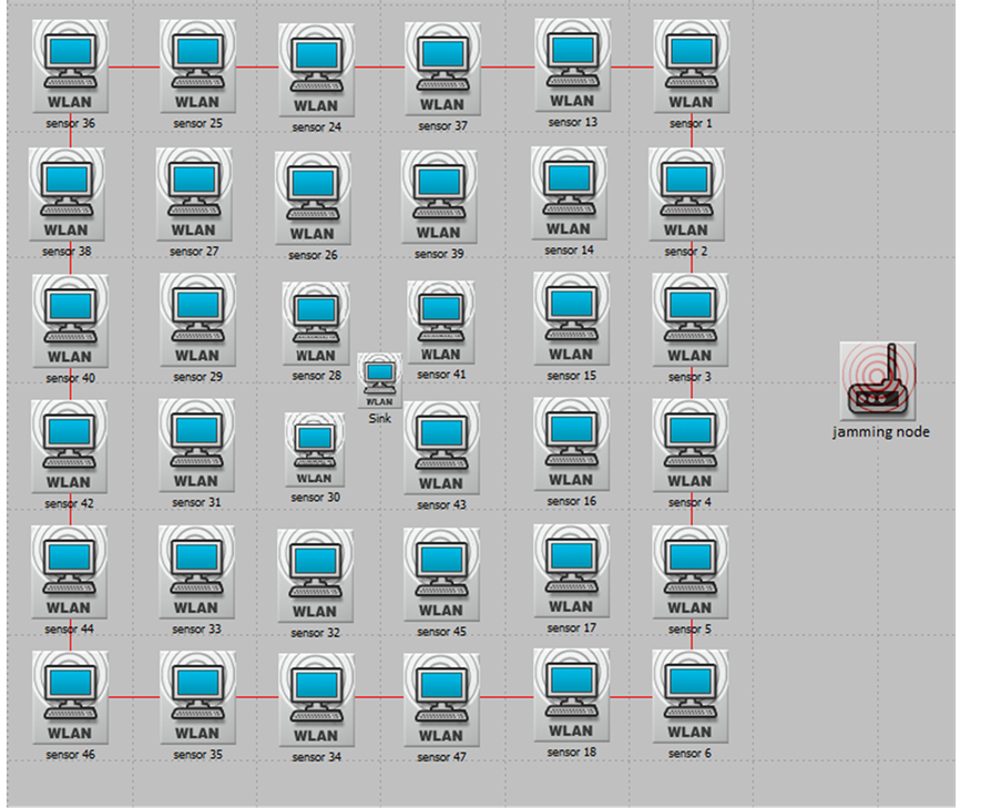
Figure 1. OPNET model with 36 nodes and a Jammer to model interference.

Table 1. ZigBee model specifications.
Table 2. Wi-Fi and low power Wi-Fi model specifications.
Table 3. Node current specifications.
In order to model the interference effects present in typical WSNs, a jammer node is utilized. As Figure 1 shows, the jammer node is placed 40 m away from the sink, thus simulating the interference caused by a neighboring network operating at the same frequency within the ISM band. As it is evident from the methodology, the simulations examine the performance of the WSN deploying either IEEE 802.15.4 or IEEE 802.11b. It is worth noting however, that the methodology is generic and can be applied to any number of nodes and any IEEE 802.11 variant. In addition, it can be applied to any node distribution. However, the choice of this standardized case study is to test the validity of this methodology against predictable results.
For all the simulations conducted, the duration is 1800 seconds and the sensor nodes transmit a 100 byte payload. Another parameter that has been varied throughout the various simulations is the packet generation rate of the nodes. The developed model was used to contrast different packet generation rates of 2, 1, 0.5 and 0.25 packets per second. As for the jammer, to account for the memory-less random nature of interference, an exponential inter-arrival time of packets with the values of 0.01 and 0.05 seconds are used. The jammer transmitting power is kept constant throughout the simulations having a value of 0.1 Watts.
To account for the inherent non-deterministic nature of CSMA/CA, 33 seeds have been conducted for each simulation and results are obtained with a confidence level of 95%.
4. Results and Discussion
In order to provide a detailed analysis of the various protocols utilized in the system, the following parameters are acquired from the simulations: the number of packets retransmitted, data dropped and the total data transmitted over the simulation time. The data collected from OPNET were incorporated into a MATLAB program implementing Equations (1) to (5) discussed in the methodology to obtain the energy consumed by the system over the given simulation duration taking into account the node contention as well as retransmissions due to collisions and interference.
As mentioned in Section 3, the impact of interference on a WSN is modeled by a jamming node operating at the ISM band. The intensity of that interference is varied by tuning the jamming node’s packet inter-arrival time. This is the periodic time interval between each successive packet generated by the jamming node. To that end, the study conducted in [8] has been extended to account for the effects of interference on each of the protocols. Figure 2 and Figure 3 demonstrate the Goodput per Joule versus system packet generation rates for two different values of jammer packet inter-arrival time. The jammer node’s packet inter-arrival times are as follows: 0.05 and 0.01 seconds. These two values for the jammer node have been chosen because OPNET simulations indicate that these values result in significant effect on the network, thus taking into account a worst-case scenario analysis. ZigBee demonstrates negative slopes in each of the two figures; while Wi-Fi and Low Power Wi-Fi have positive slopes. The reason for the positive slopes can be attributed to the sleep energy. Specifically, observing one cycle of any sensor node, it is evident that the node spends most of the cycle sleeping and only a small fraction of the cycle transmitting/receiving. Although the sleep current is much smaller than the transmitting and receiving currents it is however multiplied by a longer time period according to (1) which in turn makes the sleep energy constitute the dominant term in the energy summation. Accordingly, as the packet generation rate increases, the node sends more data over a fixed period of time resulting in a smaller sleep time. Examining Equation (6) further clarifies this behavior. As the packet generation rate increases, the total data sent along with the energy consumed increase. However, the rate at which energy consumption increases is smaller since the decrease in sleep energy counteracts the increase in transmission and reception energy. Therefore, effectively, the Goodput per Joule increases as the packet generation rate increases, thus explaining the positive slopes observed in Wi-Fi and Low Power Wi-Fi. As for the performance deterioration of ZigBee, this can be attributed to the amount of data dropped by the ZigBee nodes. As previously illustrated in [8] , nodes implementing the ZigBee protocol experience dropped data, even in the absence of noise, due to their low transmission rates.
Focusing on the performance of ZigBee under the effect of interference, a rapid deterioration can be observed implying that it is not as resilient to noise as its counterparts. Comparing Figure 4 and Figure 5 highlights this difference in immunity to interference. Figure 4 demonstrates ZigBee Goodput per Joule in different interference environments. As the jammer packet generation rate increases, ZigBee Goodput per Joule declines drastically throughout the different scenarios. Whereas observing Wi-Fi performance under interference effects in
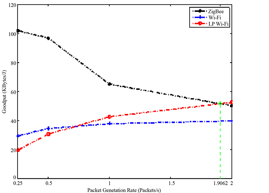
Figure 2. Goodput per Joule versus packet generation rate under the effect of interference with a jammer packet inter-arrival time of 0.05 second.
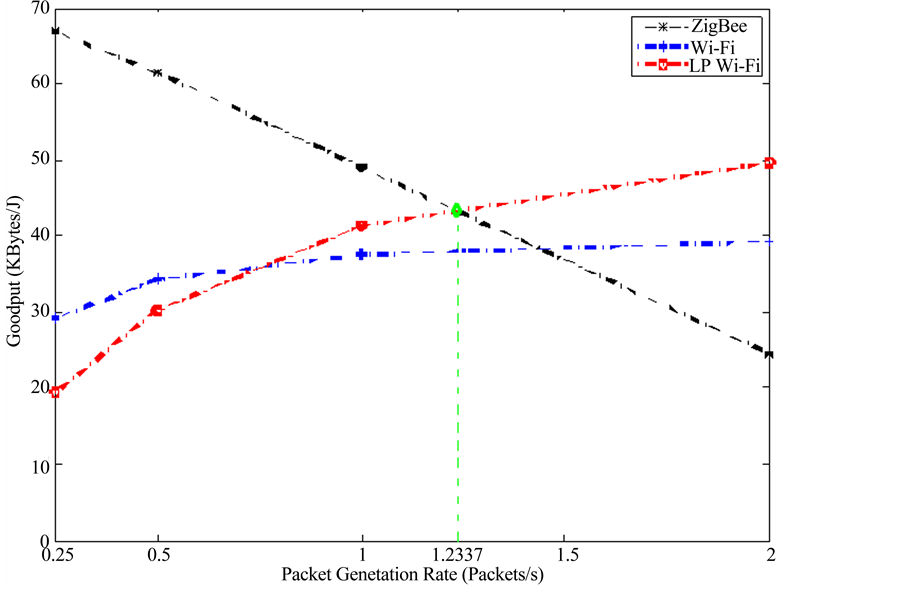
Figure 3. Goodput per Joule versus packet generation rate under the effect of interference with a jammer packet inter-arrival time of 0.01 second.
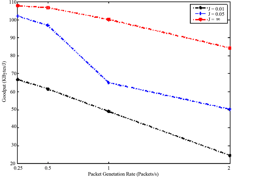
Figure 4. Goodput per Joule versus packet generation rate for ZigBee under the effect of interference with varying jammer packet inter-arrival time (J) given in seconds.
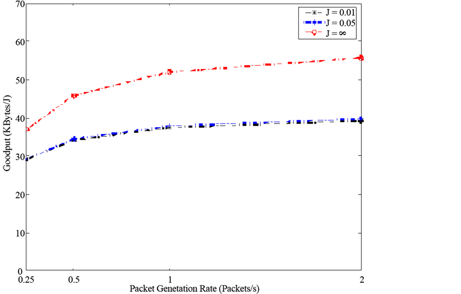
Figure 5. Goodput per Joule versus packet generation rate for Wi-Fi under the effect of interference with jammer packet inter-arrival time (J) given in seconds.
Figure 5 demonstrates that the change in packet generation rate of the jammer node seems to slightly affect Wi-Fi performance. Wi-Fi exhibits a significant difference in performance between an interference-free versus an interference heavy environment. Wi-Fi nodes must perform retransmissions, to account for the data corrupted by the jammer node. Consequently, Wi-Fi nodes consume more power for the same amount of packets transmitted, thus decreasing the Goodput per Joule. However, as the packet arrival rate of the jammer increases, the difference in behavior is insignificant. It was also found that Low Power Wi-Fi shows a similar trend to that shown by Wi-Fi yet with a slight improvement in Goodput per Joule.
Additionally, Figure 2 and Figure 3 highlight the difference in performance between ZigBee and the other two protocols. In Figure 3, the intersection point is shifted to the left indicating that as the jammer packet generation rate increases, Wi-Fi and Low Power Wi-Fi outperform ZigBee at lower node packet generation rates. The interference introduced to the system corrupts much of the data sent to the sink, which in turn causes the sink node to request a retransmission. As there is a maximum number of retransmissions defined by the ZigBee standard [10] , the node will have to eventually drop its data, causing ZigBee to be highly intolerant to interference effects.
The low data rate utilized that qualifies ZigBee as an efficient low power protocol is exactly what causes it to drop data and disqualify it as a system that is immune to interference. Accordingly, it is worth concluding that depending on the application in which the WSN is deployed, the trade-offs of each protocol need to be thoroughly studied in order to come up with the most suitable implementation. Consequently, this paper introduces a figure of merit that would aid in providing the optimum implementation solution to a given application. The figure of merit being introduced is Ξ and it is given by:
 (7)
(7)
where N is the weighting factor. Ξ puts different weights on throughput and energy efficiency depending on the value of N chosen. In other words, if it is set that N = 1, then both the throughput of the system and its energy efficiency are equally weighted and no priority is given to either parameter. Whereas, if N > 1, this indicates that the deployed system favors energy efficiency over throughput. Systems in which data loss is not critical are a good example of such a case. A specific case would be a system where data are sent repeatedly, like periodic temperature measurement, where one packet dropped is not disastrous. This is even more apparent if system lifetime is a priority. Conversely, if N < 1, this signifies that throughput is prioritized over energy efficiency. In systems in which data integrity is of key concern and battery life time is not an issue, the weighting factor is chosen to be less than unity.
5. Conclusions
This paper proposes a flexible methodology for evaluating the efficiency of a WSN while accounting for node contention, retransmissions and collisions triggered by interference effects. The efficiency is mainly defined by two parameters: energy consumption and throughput. The study was conducted using existing wireless communication standards: IEEE 802.11 and 802.15.4. A figure of merit, Ξ, is introduced. The developed figure of merit assigns different weights to energy consumption and throughput according to a given application thereby producing a methodology to aid in selecting the optimum protocol, according to application requirements. The figure of merit can be applied for systems in the absence and in the presence of interference. The proposed methodology takes into consideration data retransmitted and dropped by sensor nodes due to collisions on a given channel as well as the energy consumed by a WSN under various interference effects.
It was found that no standard is “better” than the other, but rather each standard is more fit in terms of efficiency according to application requirements. Wi-Fi and Low Power Wi-Fi are shown to be more resilient to interference, due to the use of a higher transmission power than their counterpart and hence making them more immune to interference effects. On the other hand, ZigBee uses lower transmission power, which makes it a better candidate for applications in which the emphasis is on low energy consumption under minimal noise. ZigBee would, on the contrary, perform poorly in applications where data integrity is of key significance, for ZigBee drops a lot more data, especially in high data traffic applications. Accordingly, ZigBee is not preferred in applications with low redundancy. Furthermore, it has been shown that Wi-Fi and Low Power Wi-Fi are considered to be optimum candidates for heavy traffic WSN applications. Since both (Wi-Fi and Low Power Wi-Fi) protocols provide a greater Goodput per Joule as they drop no data in the studied WSN cases, they are more suitable for applications which cannot endure any data losses.
In conclusion, this paper highlights the trade-off between energy consumption and throughput. These two parameters have inversely proportional relationships. Accordingly priorities need to be defined before deploying a given protocol. In fact, according to the defined priorities, decisions are made as to which protocol would be the most suitable. Future work will utilize the proposed methodology to investigate the tradeoffs in key WSN’s applications.
References
- Mansouri, M., et al. (2010) Factors that May Influence the Performance of Wireless Sensor Networks. In: Tan, Y.K., Ed., Smart Wireless Sensor Networks, Intech Publishing, Rijeka, 29-48.
- Li, L., Hu X.G., Chen, K. and He, K.T. (2011) The Applications of WiFi-Based Wireless Sensor Network in Internet of Things and Smart Grid. Proceedings of 6th IEEE Conference on Industrial Electronics and Applications, Beijing, 21-23 June 2011, 789-793.
- Al-Jemelim, N., Hussin, F. and Yap, V. (2010) MAC and Mobility in Wireless Sensor Networks. In: Tan, Y.K., Ed., Wireless Sensor Networks: Application-Centric Design, Intech Publishing, Rijeka, 1-23.
- Cabezas, A.C., Pena T., N.M. and Labrador, M.A. (2009) An Adaptive Multi-channel Approach for Real-Time Media Wireless Sensor Networks. Proceedings of Latin-American Conference on Communications, Medellin, 10-11 September 2009, 1-6. http://dx.doi.org/10.1109/LATINCOM.2009.5305150
- Heinzelman, W.B., Chandrakasan, A.P. and Balakrishnan, H. (2002) An Application-Specific Protocol Architecture for Wireless Microsensor Networks. IEEE Transactions on Wireless Communications, 1, 660-670. http://dx.doi.org/10.1109/TWC.2002.804190
- Yang, Z. and Mohamed, A. (2011) Wireless Sensor Networks Applications via High Altitude Systems. In: Foerster, A. and Foerster, A., Eds., Emerging Communications for Wireless Sensor Networks, Intech Publishing, Rijeka, 14-24.
- Bayraktaroglu, E., et al. (2008) On the Performance of IEEE 802.11 under Jamming. Proceedings of the 27th Conference on Computer Communication, Phoenix, 13-18 April 2008, 1265-1273.
- Kenawy, A., et al. (2013) WSN Goodput and Energy Consumption for Various Wireless Communication Standards. Proceedings of the International Conference on Technological Advances in Electrical, Electronics and Computer Engineering, Konya, 9-11 May 2013, 40-45.
- (1997) IEEE Std. 802.11.
- (2008) IEEE Std. 802.15.4.
- OPNET Official Website. http://www.opnet.com
- Casilari, E., Cano-Garci, J.M. and Campos-Garrido, G. (2010) Modeling of Current Consumption in 802.15.4/ZigBee Sensor Motes. Sensors, 10, 5443-5468. http://dx.doi.org/10.3390/s100605443
- Ting, K., Kuo, F., Hwang, B., Wang, H. and Lai, F. (2010) An Accurate Power Analysis Model Based on MAC Layer for the DCF of 802.11n. Proceedings of the 12th IEEE International Symposium on Parallel and Distributed Processing with Applications, Taipei, 6-9 September 2010, 350-358. http://dx.doi.org/10.1109/ISPA.2010.88
- Kim, T., Park, J., Chong, H., Kim, K. and Choi, B. (2008) Performance analysis of IEEE 802.15.4 Non-Beacon Mode with the Unslotted CSMA/CA. IEEE Communication Letters, 12, 238-240. http://dx.doi.org/10.1109/LCOMM.2008.071870
- Chen, J., Sivalingam, K.M., Agrawal, P. and Kishore, S. (1998) A Comparison of MAC Protocols for Wireless Local Networks Based on Battery Power Consumption. Proceedings of the 17th Conference on Computer Communication. San Francisco, 29 March-2 April 1998, 150-157.