Wireless Sensor Network
Vol.6 No.2(2014), Article ID:43028,8 pages DOI:10.4236/wsn.2014.62003
Quality of Service in Wireless Sensor Networks
1The Nelson Mandela African Institution of Science and Technology, School of Computational Science and Communication Engineering, Arusha, Tanzania
2Faculty of Economic Science and Information Technology, TIRDO/North West University, Vanderbijlpark, South Africa
Email: mbowej@nm-aist.ac.tz, george.oreku@gmail.com
Copyright (c) 2014 Joseph E. Mbowe, George S. Oreku. This is an open access article distributed under the Creative Commons Attri-bution License, which permits unrestricted use, distribution, and reproduction in any medium, provided the original work is properly cited. In accordance of the Creative Commons Attribution License all Copyrights (c) 2014 are reserved for SCIRP and the owner of the intellectual property Joseph E. Mbowe, George S. Oreku. All Copyright (c) 2014 are guarded by law and by SCIRP as a guardian.
Received October 21, 2013; revised November 21, 2013; accepted November 28, 2013
Keywords:Wireless Sensor Network; QoS; Probability; Metrics; Serviceability
ABSTRACT
The growing demand of usage of wireless sensors applications in different aspects makes the quality-of-service (QoS) to be one of paramount issues in wireless sensors applications. Quality of service guarantee in wireless sensor networks (WSNs) is difficult and more challenging due to the fact that the resources available of sensors and the various applications running over these networks have different constraints in their nature and re- quirements. Traditionally quality of service was focused on network level with concern in metrics such as delay, throughput, jitter e.c.t. In this paper we present appropriate metrics of QoS for WSN which involve service, re- liability and availability which ultimately facilitating in archiving qualitable service. We discuss the reverse look of QoS and hence present mathematically the three significant quality factors that should currently be taken into account in developing WSNs application quality services namely, availability, reliability and serviceability. We run experiments incorporating these three phenomenons (reliability, availability and serviceability—RAS) to demonstrate how to attain QoS which effectively improve reliability of the overall WSNs.
1. Introduction
Quality of service is an overused term with multiple meanings and perspectives from different research and technical communities [1]. QoS in WSNs can be viewed from two perspectives: application-specific and network. The former refers to QoS parameters specific to the application, such as sensor node measurement, deployment, and coverage and number of active sensor nodes. The latter refers to how the supporting communication network can meet application needs while efficiently using network resources such as bandwidth and power consumption.
With the recent technological developments of the wireless networks and multifunctional sensors with processing and communication capabilities, wireless sensor networks (WSNs) have been used in an increasing number of applications. WSNs can provide a more accurate or reliable monitoring service for different classes of applications [2,3]. Quality of service can be an important mechanism to guarantee that the distinct requirements for different classes of applications are met [4].
Traditional QoS mechanisms used in wired networks aren’t adequate for WSNs because of constraints such as resource limitations and dynamic topology. One of the many challenges concerning wireless sensor networks (WSNs) is how to provide Quality of Service (QoS) parameter guarantees in real-time applications [5]. Therefore, middleware should provide new mechanisms to maintain QoS over an extended period and even adjust itself when the required QoS and the state of the application changes. Middleware should be designed based on trade-offs among performance metrics such as network capacity or throughput, data delivery delay, and energy consumption in order to provide QoS in Wireless Sensor Network.
1.1. QoS Concept
As defined in [6], Quality-of-Service is a set of service requirements to be met by the network while transporting a flow. “Here a flow is” a packet stream from source to a destination (unicast or multicast) with an associated Quality of Service (QoS) [6]. In other words, QoS is a measurable level of service delivered to network users, which can be characterized by packet loss probability, available bandwidth, end-to-end delay, etc. Such QoS can be provided by network service providers in terms of some agreement (Service Level Agreement, or SLA) between network users and service providers. For example, users can require that for some traffic flows, the network should choose a path with minimum 2M bandwidth.
1.2. QoS Metrics
For quality of service to be implemented, service requirements have to be expressed in some measurable QoS metrics. The well-known metrics include bandwidth, delay, jitter, cost, loss probability, etc. Different metrics may have different features. There are 3 types of metrics when talking about QoS: additive, multiplicative, and concave [7]. These can be defined as follows:
Let m (n1, n2) be a metric for link (n1, n2). For any path P = (n1, n2, ···, ni, nj), metric m is: (Note here n1, n2, n3, ···, ni, nj represent network nodes)
additive, if m (P) = m (n1, n2) + m (n2, n3) + ··· + m (ni, nj)
Examples are delay, jitter, cost and hop-count. For instance, the delay of a path is the sum of the delay of every hop.
multiplicative, if m (P) = m (n1, n2) * m (n2, n3) * ··· * m (ni, nj)
Example is reliability, in which case 0 < m (ni, nj) < 1.
concave, if m (P) = min {m (n1, n2), m (n2, n3), ···, m (ni, nj)}
Example is bandwidth, which means that the bandwidth of a path is determined by the link with the minimum available bandwidth.
2. QoS Challenges in Sensor Networks
Different from IP network, Sensor network naturally supports multiple service types, thus provides different QoS. The service types range from CBR (Constant Bit Rate) which guarantees bandwidth, delay and delay jitter, to UBR (Unspecified Bit Rate) which virtually provides no guarantees (just like today’s “best-effort” IP network). While sensor networks inherit most of the QoS issues from the general wireless networks, their characteristics pose unique challenges. The following is an outline of design considerations for handling QoS traffic in wireless sensor networks.
Bandwidth limitation: A typical issue for general wireless networks is securing the bandwidth needed for achieving the required QoS. Bandwidth limitation is going to be a more pressing issue for wireless sensor networks. Traffic in sensor networks can be burst with a mixture of real-time and non-real-time traffic. Dedicating available bandwidth solely to QoS traffic will not be acceptable. A trade-off in image/video quality may be necessary to accommodate non-real-time traffic. In addition, simultaneously using multiple independent routes will be sometime needed to split the traffic and allow for meeting the QoS requirements. Setting up independent routes for the same flow can be very complex and challenging in sensor networks due energy constraints, limited computational resources and potential increase in collisions among the transmission of sensors.
Removal of redundancy: Sensor networks are characterized with high redundancy in the generated data. For unconstrained traffic, elimination of redundant data messages is somewhat easy since simple aggregation functions would suffice. However, conducting data aggregation for QoS traffic is much more complex. Comparison of images and video streams is not computationally trivial and can consume significant energy resources. A combination of system and sensor level rules would be necessary to make aggregation of QoS data computationally feasible. For example, data aggregation of imaging data can be selectively performed for traffic generated by sensors pointing to same direction since the images may be very similar. Another factor of consideration is the amount of QoS traffic at a particular moment. For low traffic it may be more efficient to cease data aggregation since the overhead would become dominant. Despite the complexity of data aggregation of imaging and video data, it can be very rewarding from a network performance point-of-view given the size of the data and the frequency of the transmission.
Energy and delay trade-off: Since the transmission power of radio is proportional to the distance squared or even higher order in noisy environments or in the nonflat terrain, the use of multi-hop routing is almost a standard in wireless sensor networks. Although the increase in the number of hops dramatically reduces the energy consumed for data collection, the accumulative packet delay magnifies. Since packet queuing delay dominates its propagation delay, the increase in the number of hops can, not only slow down packet delivery but also complicate the analysis and the handling of delay-constrained traffic. Therefore, it is expected that QoS routing of sensor data would have to sacrifice energy efficiency to meet delivery requirements. In addition, redundant routing of data may be unavoidable to cope with the typical high error rate in wireless communication, further complicating the trade-off between energy consumption and delay of packet delivery.
Buffer size limitation: Sensor nodes are usually constrained in processing and storage capabilities. Multi-hop routing relies on intermediate relaying nodes for storing incoming packets for forwarding to the next hop. While a small buffer size can conceivably suffice, buffering of multiple packets has some advantages in wireless sensor networks. First, the transition of the radio circuitry between transmission and reception modes consumes considerable energy and thus it is advantageous to receive many packets prior to forwarding them. In addition, data aggregation and fusion involves multiple packets. Multihop routing of QoS data would typically require long sessions and buffering of even larger data, especially when the delay jitter is of interest. The buffer size limitation will increase the delay variation that packets incur while traveling on different routes and even on the same route. Such an issue will complicate medium access scheduling and make it difficult to meet QoS requirements.
Support of multiple traffic types: Inclusion of heterogeneous set of sensors raises multiple technical issues related to data routing. For instance, some applications might require a diverse mixture of sensors for monitoring temperature, pressure and humidity of the surrounding environment, detecting motion via acoustic signatures and capturing the image or video tracking of moving objects. These special sensors are either deployed independently or the functionality can be included on the normal sensors to be used on demand. Reading generated from these sensors can be at different rates, subject to diverse quality of service constraints and following multiple data delivery models, as explained earlier. Therefore, such a heterogeneous environment makes data routing more challenging.
3. Reliability, Availability and Serviceability
As Wireless Sensor Networks (WSNs) are expected to be adopted in many industrial, health care and military applications, their reliability, availability and serviceability (RAS) are becoming critical. In recent years, the diverse potential applications for wireless sensor networks (WSN) have been touted by researchers and the general press [8-10]. In many WSNs systems, to provide sufficient RAS can often be absorbed in the network cost. Nevertheless, as noticed early [11], network designers face “two fundamentally conflicting goals: to minimize the total cost of the network and to provide redundancy as a protection against major service interruptions.”
For availability and serviceability, remote testing and diagnostics is needed to pinpoint and repair (or bypass) the failed components that might be physically unreachable. Severe limitations in the cost and the transmitted energy within WSNs negatively impact the reliability of the nodes and the integrity of transmitted data. The application itself will greatly influence how system resources (namely, energy and bandwidth) must be allocated between communication and computation requirements to achieve requisite system performance. The presentation below demonstrates how different application wireless sensor nodes can influence the resource usability:
Power states are states of particular devices; as such, they are generally not visible to the user. For example, some devices may be in the Off state even though the system as a whole is in the working state.
These states are defined very generically in this section to enable applications adopted in our approach. Many devices do not have all four power states defined. Devices may be capable of several different low power modes, but if there is no user-perceptible difference between the modes only the lowest power mode will be used. We define four power states according to advanced configuration power interface (ACPI) [12]:
Ready—(or busy) is when the system or device is fully powered up and ready for use.
Idle—is an intermediate system dependent state that attempts to conserve power. The CPU enters the idle state when no device activity has occurred within a machine defined time period. The machine won’t return to busy state until a device raises a hardware interrupt or the machine accesses a controlled device.
Suspend—is the lowest level of power consumptions available in which memory preserves all data and operational parameters. The device won’t perform any computations until it resumes normal activity, which it does when signal by an external event such as a button press, timer alarm, or receipt of request.
When Off—the device is powered down and inactive. Operational and data parameters might or might not be preserved in
Figure 1 shows the general current ranges for each
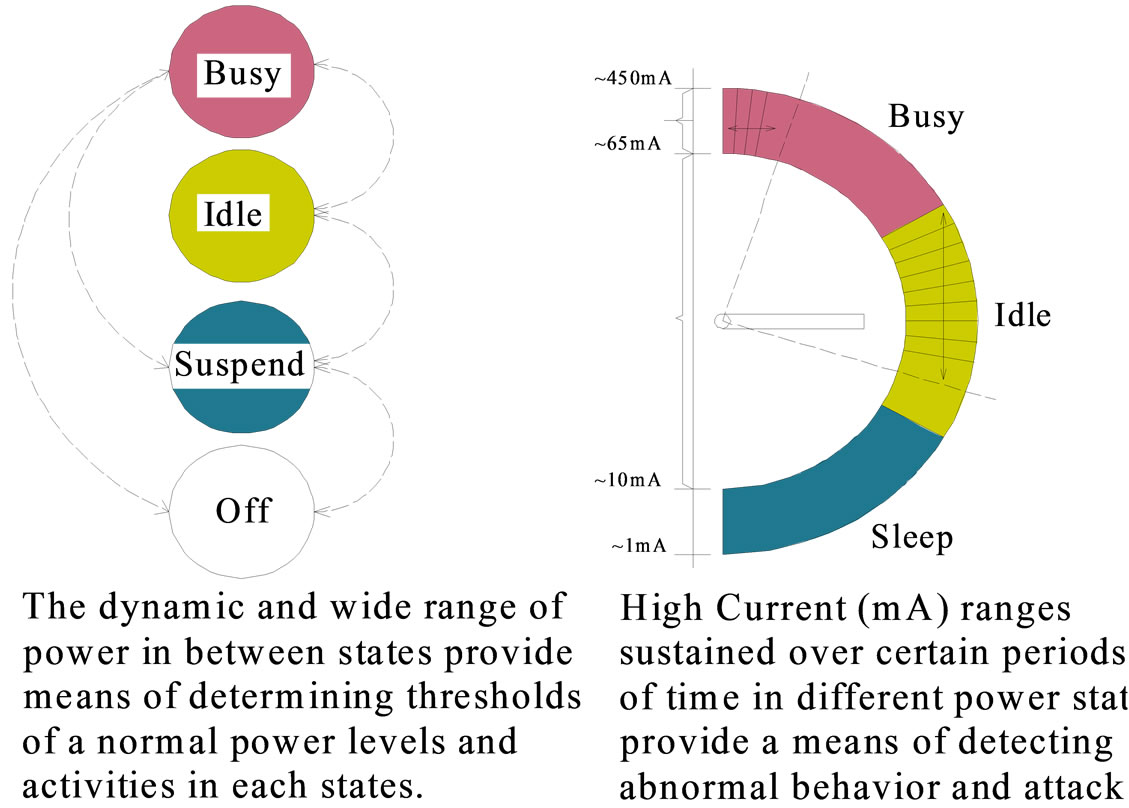
Figure 1. State power distribution (adapted from a Dell Axim) and battery-based intrusion detections (B-BID) power drain rate thresholds. The longer a threshold is held high in the busy and idle states, the greater the likehood that an anomalous activity is present.
operating state as well as the power distribution for a PDA class of devices. Cliff Brake affirms that the CPU accounts for approximately 30 percent of power and the screen 42 percent when backlit these percentages vary slightly with each PDA class [13]. In an idle state, the CPU loses nearly all current and the backlight is turned off, equating to an approximate 64 percent power reduction.
This can be deceiving, however. In idle state, if the wireless local area network (LAN) card picks up a network request and transmits an acknowledgement, the CPU will consume power at a higher level. Worse yet, once on, the card might pick up multiple requests, and unless the user has altered the CPU’s communication protocol, it will try to send multiple acknowledgements for each request. In addition, the power required to transmit is greater than it is to receive by approximately 1.5:1 [14,15].
The justification of idle state resource consumption can be only identified through worse or best scenarios as follow:
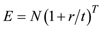 (1)
(1)
The inputs are the total number of nodes (N), threshold (r), the time taken (t), and total time (T). One of the purposes of a model such as this is to make predictions and try “What If?” scenarios. You can change the inputs and recalculate the model and you’ll get a new answer. You might even want to plot a graph of the expected results (E) vs. time (T). In some cases, you may have a fixed results rate, but what do you do if the results rate is allowed to change? For this simple equation, you might only care to know a worst/best case scenario, where you calculate the expected value based upon the lowest and highest results rates that you might expect.
While examining WSN nodes and propose the necessary QoS required for increasing both the availability and serviceability of the system our approach is service oriented and was particularly motivated by recent proposals to define QoS (quality of service) for WSN. In one definition, QoS measures application reliability with a goal of energy efficiency [16]. An alternative definition equates QoS to spatial resolution [17]. This latter work also presented a QoS control strategy based on a Gur game paradigm in which base stations broadcast feedback to the network’s sensors. QoS control is required for the assumption is that the number of sensors deployed exceeds the minimum needed to provide the requisite service.
This work presents two new techniques to maintain QoS under a variety of network constraints. We first adapt the proposed Gur game strategy to operate in energy poor environments then proposes a new, extremely low-energy control strategy based on individual feedback in a random access communication system. In particular, our work is applicable to networks that are deployed in remote, harsh environs (e.g., space applications). Such networks are constrained by (1) high die-off rates of nodes and (2) inability to be replenished. The performance of the proposed algorithms is demonstrated throughout using numerical examples as follows (2) and (3):
 (2)
(2)
Where m is a number of failed nodes within WSN.
n is number of nodes within WSN and  is possible percentage of failed nodes within given WSN.

4. Calculating Probability of Nodes Availability in WSN
The availability of several implementations is derived from Equation (3) above for Mean Time between Failure (MTBF) and Mean Time to Repair (MTTR). Due to the power issue and the unpredictable wireless network characteristics, it is possible that applications running on the sensor nodes might fail. Thus, techniques to improve the availability of sensor nodes are necessary. Estimated MTBF in our sensor nodes is based on the individually calculated failure rates for each component and the circuit board. Next, for the redundant system versions, if the failure rates (λ) of each redundant element are the same, then the MTBF of the redundant system with n parallel independent elements (i) [18] are taken as:
 (4)
(4)
The MTTR can be estimated by the sum of two values, referred to as Mean Time to Detect (MTTD) the failures and the Time to Repair (TTR) (MTTR = MTTD + TTR). Notice that this part might be severely affected by the network connections.
| |
Considering the technique [19], where the consumer starts the reparation mechanism by activating the local functional test. Once it completes, the test result is sent back to the consumer for analysis. If a failure occurs, the consumer will send the repair message to the sensor node and initialize the backup component. Acknowledgement is sent back to the consumer once the reparation is completed. If the message latency from the consumer to the target node is d seconds and the test time is c seconds, then we calculate MTTR as Equation (5):
 (5)
(5)
For the sensor node without the Test Interface Module [19], consumer sends the measured data request command to the suspected sensor node. In order to check the data integrity, same request command will also send to at least two other nearby sensor nodes. The consumer compares the three collected streams of data and pinpoints the failed node. Once the failure is confirmed, consumer will notify the surrounding sensor node to take over the applications of the failed node. Once the failure is confirmed, consumer will notify the surrounding sensor node to take over the applications of the failed node. Again if the message latency from the consumer to the target node is d seconds, then MTTR is:
 (6)
(6)
To estimate realistic MTTR numbers, we use study [20], where for WSNs Thermostat application with 64 sensor nodes is simulated. Due to the power and protocol requirements, the average latency of related messages is 1522s. By applying this to our MTTR estimations, the test time c is much smaller and can be neglected.
Reliability of a system is defined as the probability of system survival Equation (7) in a period of time. Therefore, using Poisson probability [21] implemented for WSNs we have as well estimate probability of “failed” situation for whole WSN in given time interval, e.g. for one day (24 hours) to demonstrate the reliability of our presented approach.
 (7)
(7)
Where Probability (r) is a probability of failure system working with “r” failed nodes within WSN for given time interval,  , m is a average number of failed nodes within WSN and e = 2.718…
For example, in average there are 3 failed nodes in WSN fo 24 hours. Then we calculate Probabilities of failure system working as:

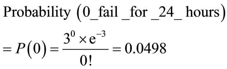
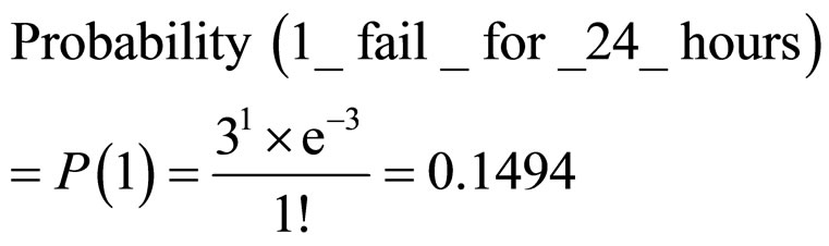
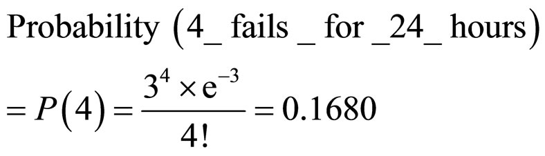
From this example, we can see that with progressive increase of fail nodes quantity of a WSN, the risk of unstable work also increases.
5. Experiments and Evaluation
The discussion in this section will be about achieving two primary factors of dependability in WSNs applications, namely availability and reliability. In the classical definition, a system is highly available if the fraction of its downtime is very small, either because failures are rare, or because it can restart very quickly after a failure [22].
The performance of the proposed approach is demonstrated throughout using numerical examples. Reliability of a system is defined as the probability of system survival in a period of time. Since it depends mainly on the operating conditions and operating time, the metrics of Mean Time between Failure (MTBF) is used. For time period of duration t, MTBF is related to the reliability as follows [19]:
 (8)
(8)
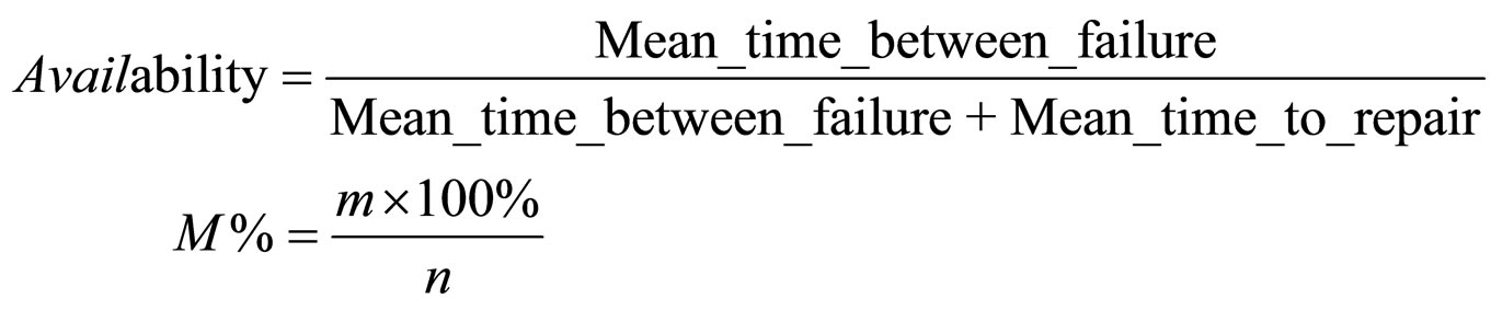
Availability of a system is closely related to the reliability, since it is defined as the probability that the system is operating correctly at a given time. Dependence availability and reliability on MTBF presented on Figure 2. Calculating availability is related to MTBF and Mean Time to Repair (MTTR) by the following relation [19]:
 (9)
(9)
Considering availability of each node in isolation, from Equation (9), the MTTR should be minimized, while MTBF should be maximized. While MTBF is given by manufacturing practices and components used, the value of MTTR can be controlled by both individual node and network design.
 (10)
(10)
where m is a number of failed nodes within WSN, n is number of nodes within WSN and  is possible percentage of failed nodes within given WSN.
Serviceability of a system is defined as the probability that a failed system will restore to the correct operation. Serviceability is closely related to the repair rate and the MTTR [19].
 (11)
(11)
A fundamental service in sensor networks is the determination of time and location of events in the real world. This task is complicated by various challenging characteristics of sensor networks, such as their large scale, high network dynamics, restricted resources, and restricted energy. We use Hawk sensor nodes for determination time of data transmitting in fulfilling the QoS under these constraints. We illustrate the practical feasibility to our approaches by concrete application of real sensor nodes (Hawk Sensor Nodes) to our experiments and the results of availability and reliability of sensor nodes to reveal QoS from our experiment can be seen on Figure 2 above.
In any system one must consider the reliability of its components when ascertaining overall system performance. Thus our question was whether the proposed strategy performed adequately for various levels of sensor reliability. Equation (2), does not include any information regarding expected sensor life and thus assumes static network resources, which is clearly not the case in WSNs. For example, sensors may fail at regular intervals due to low reliability, due to cost driven design choices, environmentally caused effects (especially in harsh environments), loss of energy, etc.
We measured the processing throughput, i.e., the number of data transmitted events that each phase is able to process per second and time taken to transmit these data within selected sensor nodes, as can be seen in graph presentation in Figure 3.
We plot the node availability versus average latency, which lumps together the characteristics of the channel, the number of retransmission retries on the failure, as well as the node-dependent features such as retransmission timeouts in Figure 4.
In Figure 5, we examine WSNs nodes to transmit the data in evaluating (RAS). Two sensor nodes with 32 size byte were used for estimating connection time with different transmitting rate. With 0.0625 t/s, we were able to connect 32 packets. To ask one sensor node to transmit the data we need 2 data packets (one for asking, another one for receiving the answer). To estimate Time to connection we have to transmit only two packets. Number of packets = file size/packet size. Time = number of packets/ data transmitting rate. This can be used to propose the necessary infrastructure required for increasing both the availability and serviceability of the system, in spite of the absence of a reliable transport layer. Hence this can be used to analyze and detect delay, delivery, perfor-
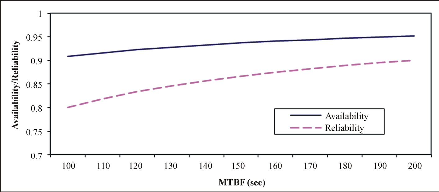
Figure 2. Dependence availability and reliability on MTBF.
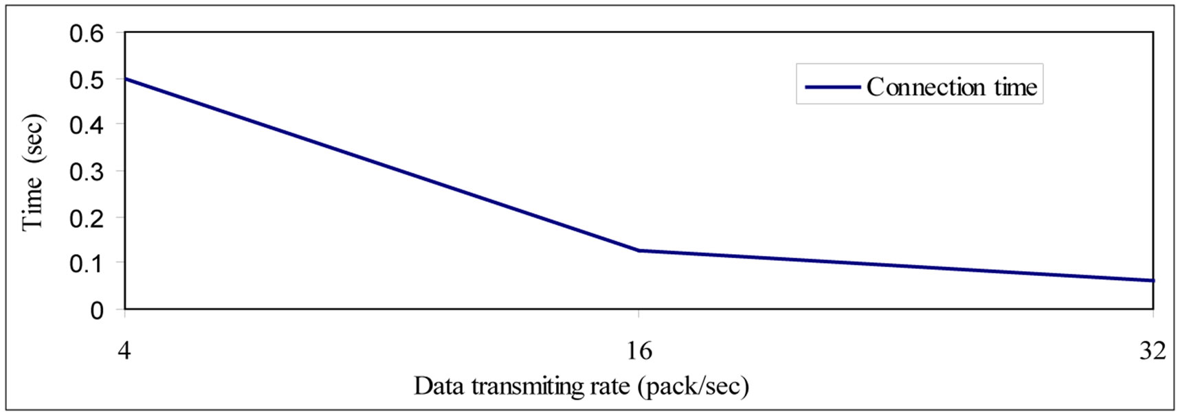
Figure 3. Connection time for 4/16/32 pack/sec.
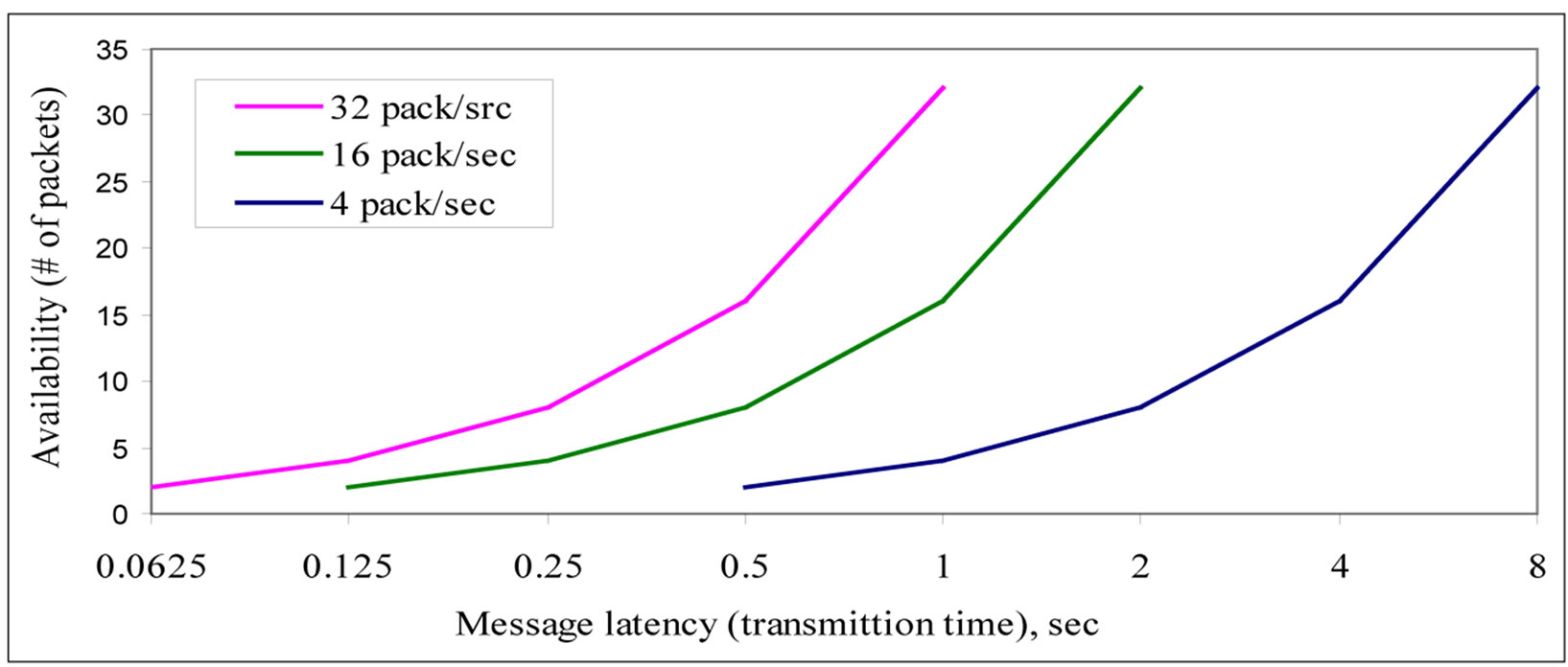
Figure 4. Availability of a Node in WSN.
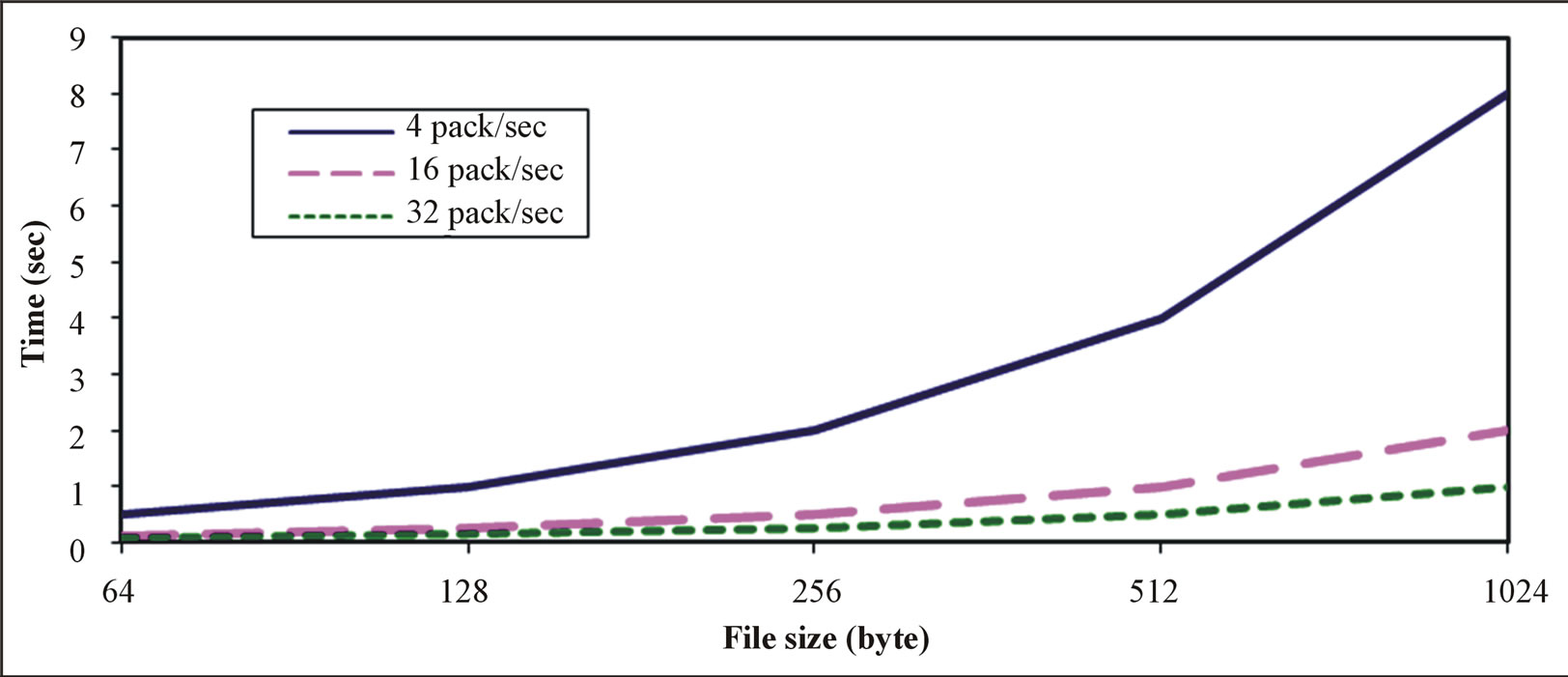
Figure 5. Transmitting time in different number of packets to access (RAS).
mance or energy consumptions.
6. Conclusions
One primordial issue in WSN is to satisfy application QoS requirements while providing a high-level abstraction that addresses good service. Notice that although we consider primarily testing in the laboratory, the proposed solutions can easily be applied to testing in factory with large size of Sensor network applications.
With the proposed approach, such tests can be easily parallelized by applying wireless broadcast to many nodes at once. As a result, the proposed approach can be used in variety of testing scenarios.
In this paper, QoS in WSN has been proposed through reliability availability and serviceability metrics, Using mentioned components we have evaluated QoS and system-level test using sensor nodes.
However our finding found that effects of traditional metrics (delay, throughput, jitter e.c.t.) place a lot of burden on the QoS of the overall system thus decreasing performance.
REFERENCES
- D. Chen and P. K. Varshney, “QoS Support in Wireless Sensor Networks: A Survey,” Proceedings of the International Conference on Wireless Networks (ICWN 04), Las Vegas, 21-24 June 2004, pp. 227-233.
- J. Yick, B. Mukherjee and D. Ghosal, “Wireless Sensor Network Survey,” Computer Networks, Vol. 52, No. 12, 2008, pp. 2292-2330. http://dx.doi.org/10.1016/j.comnet.2008.04.002
- J. L. Lu, W. Shu and W. Wu, “A Survey on Multipacket Reception for Wireless Random Access Networks,” Journal of Computer Networks and Communications, Vol. 2012, 2012, 14 p.
- D. Chen and P. K. Varshney, “QoS Support in Wireless Sensor Networks: A Survey,” Proceedings of the International Conference on Wireless Networks, Las Vegas, 2004, pp. 609-619.
- M. Z. Hasan and T. C. Wan, “Optimized Quality of Service for Real-Time Wireless Sensor Networks Using a Partitioning Multipath Routing Approach,” Journal of Computer Networks and Communications, Vol. 2013, 2013, 18 p. http://dx.doi.org/10.1155/2013/497157
- E. Crawley, R. Nair, B. Rajagopalan and H. Sandick, “A Framework for QoS-Based Routing in the Internet,” RFC 2386, Internet Eng. Task Force, 1997. fttp://fttp.ietf.org/internet-draftsdraft-ietf-qosr-framework-02.txt
- S. G. Chen, “Routing Support for Providing Guaranteed End-to-End Quality-of-Service,” Ph.D. Thesis, University of Illinois at Urbana-Champaign (UIUC), Champaign, 1999. http://cairo.cs.uiuc.edu/papers/SCthesis.ps.
- G. Pottie and W. Kaiser, “Wireless Integrated Network Sensors,” Communications of the ACM, Vol. 43, No. 5, 2000, pp. 51-58. http://dx.doi.org/10.1145/332833.332838
- D. Estrin, L. Girod, G. Pottie and M. Srivastava, “Instrumenting the World with Wireless Sensor Networks,” Proceedings of International Conference Acoustics, Speech and Signal Processing (ICASSP 2001), May 2001, pp. 2675-2678.
- MIT Technology Review, “10 Emerging Technologies That Will Change the World,” MIT’s Magazine of Innovation Technology Review, 2003. www.technologyreview.com
- R. F. Rey, “Engineering and Operations in the Bell System,” Bell Labs, Murray Hill, 1977.
- X. Wang, W. Gu, K. Schosek, S. Chellappan and D. Xuan, “Sensor Network Configuration under Physical Attacks,” Technical Report Technical Report (OSU-CISRC-7/04- TR45), The Ohio-State University, Columbus, 2004.
- X. Wang, W. Gu, S. Chellappan, D. Xuan and T. H. Laii, “Search-Based Physical Attacks in Sensor Networks: Modeling and Defense,” Technical Report, The OhioState University, Columbus, 2005.
- H. Chan, A. Perrig and D. Song, “Random Key Predistribution Schemes for Sensor Networks,” Proceedings of the 2003 IEEE Symposium on Security and Privacy, Washington DC, 2003, p. 197.
- Y. Desmedt and S. Jajodia, “Redistributing Secret Shares to New Access Structures and Its Applications,” Technical Report ISSE TR-97-01, George Mason University, Fairfax, 1997.
- M. Perillo and W. Heinzelman, “Providing Application QoS through Intelligent Sensor Management,” 1st Sensor Network Protocols and Applications Workshop (SNPA 2003), Anchorage, 11 May 2003, pp. 93-101.
- R. Iyer and L. Kleinrock, “QoS Control for Sensor Networks,” IEEE International Communications Conference (ICC 2003), Anchorage, 11-15 May 2003, pp. 517-521.
- Arora, et al., “Extreme Scale Wireless Sensor Networking,” Technical Report, 2004. http://www.cse.ohio-state.edu/exscal/
- M. W. Chiang, Z. Zilic, K. Radecka and J.-S. Chenard, “Architectures of Increased Availability Wireless Sensor Network Nodes,” ITC International Test Conference, Vol. 43, No. 2, 2004, pp. 1232-1241.
- Headquarters, Department of the Army, “Reliability/Availability of Electrical & Mechanical Systems for Command, Control, Communications, Computer, Intelligence, Surveillance, and Reconnaissance Facilities,” Department of the Army, Washington DC, 2003.
- M. Eddous and R. Stansfield, “Methods of Decision Making,” UNITY, Audit, 1997.
- J. C. Knight, “An Introduction to Computing System Dependability,” Proceedings of the 26th International Conference on Software Engineering (ICSE’04), Scotland, 2004, pp. 730-731. http://dx.doi.org/10.1109/ICSE.2004.1317509