Wireless Sensor Network
Vol.5 No.5(2013), Article ID:31769,14 pages DOI:10.4236/wsn.2013.55012
Cross-Layer Energy Analysis and Proposal of a MAC Protocol for Wireless Sensor Networks Dedicated to Building Monitoring Systems
1XLIM Laboratory, SIC department, University of Poitiers, Poitiers, France
2Department of Health and Comfort, Centre Scientifique et Technique du Bâtiment, St Martin d’Hères, France
Email: dessales@sic.univ-poitiers.fr
Copyright © 2013 Denis Dessales et al. This is an open access article distributed under the Creative Commons Attribution License, which permits unrestricted use, distribution, and reproduction in any medium, provided the original work is properly cited.
Received March 22, 2013; revised April 23, 2013; accepted May 7, 2013
Keywords: WSN; Physical Layer; MAC Layer; Energy Consumption; Cross-Layer Analysis
ABSTRACT
In a sustainable development context, the monitoring systems are essential to study the building energy performances. With the recent technology advances, these systems can be based on wireless sensor networks, where the energy efficiency is the main design challenge. To this end, most of the studies focus on low power Medium Access Control (MAC) protocols to reduce the overall energy consumption of a network. Nevertheless, the performances assessment of these protocols is generally not performed in a realistic way, and does not take into account the performances of the other layers of the OSI model. In this paper, we propose a cross-layer methodology to assess the real performances of a MAC protocol by taking into account the traffic volume, the synchronization losses and more particularly the physical layer performances through a Bit Error Rate (BER) criterion. The simulation results demonstrate clearly the physical layer impact on a sensor lifetime. Finally, the proposal of an energy efficient MAC protocol for a wireless sensor network dedicated to an application of building monitoring is proposed.
1. Introduction
The international community has fixed as a target to halve the emissions of greenhouse gases before 2050 on the planet scale. In France, the consumption caused by the use of buildings currently represents 40% of the total energy consumed. In this goal, building monitoring systems based on Wireless Sensor Networks (WSN) are essential [1] to assess energy performances and to identify the possible actions to reduce the overall energy consumption of a building. However, the main challenge encountered in the design of a WSN concerns the energy efficiency of radio communications. This efficiency is important because in many scenarios, each sensor operates without battery replacement for several years.
Recent advances on energy efficiency for WSN are organized essentially around the optimization of the lower layers of OSI model. At the physical layer level, most of the studies [2,3] are based on the improvement of the Bit Error Rate (BER) to reduce significantly the transmission power. At the MAC layer level, the use or the design of low power MAC protocols according to the application is essential to minimize idle listening, overhearing and collisions [4,5]. Nevertheless, the performances of MAC protocols proposed in the literature are complex to assess. They depend on both the application in question and the implemented physical layer. Moreover, the MAC and physical layers are inter correlated in particular for the clock synchronization management according to the frames construction, the exchange cycle of frames and the clock PLL management. So due to this kind of interdependency, a “cross layer” analysis tends to be more efficient than a traditional separate optimization on each layer [6].
In this paper, we present a cross-layer analysis to reduce energy consumption for sensors autonomous in energy. This study is based on realistic models of physical channel and realistic energy consumption from processor and radio components. The numerical aspects are developed in the context of building monitoring.
This paper is hence organized as follows. In Section 2, we present a MAC protocol classification to express their impact on the energy consumption question. In Section 3, we describe our method to assess MAC protocols in a realistic way particularly by taking into account the physical layer performances. Then, we choose two existing MAC protocols and an ideal one to develop the analysis and compare them in Section 4. In Section 5, we propose an energy efficient protocol dedicated to building monitoring systems and we compare it to the others before to propose some new trends in Section 6.
2. Related Work on MAC Protocols
The MAC part of networks protocols is principally in charge of the channel sharing and of the frame construction and its exchange. So, according to the MAC protocol, the number and the length of exchanged frames in a time unit can greatly varied, with great consequences on the energy cost. Several communities have proposed MAC protocols adapted to public, industrial or secured networks with different kind of constraints to solve: production cost, real-time or error-less communication. In our application context, we have studied all these kinds of solutions compared to our constraints: energy consumption, temporal determinism.
To explain the impact of a MAC protocol in a cross-layer sense, we propose a classification based on Vasques work [7]. Following Vasques, we have chosen to classify the existing MAC protocols in a classification tree based on the scheduling process used for the channel access. This classification is illustrated in Figure 1.
Our idea is to link this scheduling choice with the energy consumption. The blue colour allows highlighting protocols where the scheduling process is based on assigning priorities on the message flows, and the orange colour the protocols where the scheduling process is based on an access time limited to the stations.
The decision to not control the channel access and to use contention based [8,9] or preamble sampling protocols [10,11] induces two possibilities: to accept or not the probability of frame collision. So in the first case, the impact upon the energy consumption is linked to the error probability and the energy cost of a frame. With the CSMA/CA protocol (Carrier Sense Multiple Access/ Collision Avoidance), like in CAN networks (Controller Area Networks) for example, the signal management involves that all nodes must be perfectly synchronous, with for consequences: high frequency of exchange cycles or a long preamble part in the frame, either two consequences with an impact on the energy cost.
In parallel of public networks, the industrial world has developed numerous solutions to solve particular constraints like minimal time of alarm delivery or real-time command. If the first constraint can be solved without access control, like Ethernet networks, the great majority of solutions (Profibus, ASI, WorldFIP ...) are based on controlled channel access due to the deterministic temporal constraints. Two mechanisms exist, either each node receives successively the right to send one message sequence (WorldFIP), either each node receives successsively a time delay to use for his communication (Profibus for example). Such solutions impact the energy consumption at the level of the nodes sleep/wakeup cycles. When the communication comes exactly in the expected temporal window, each node could be wake-up very precisely, by opposition, when the uncertainty is important, the node must be wake-up in advance and in listening mode during a long time.
It is also very important to see that in such industrial context, two kinds of nodes can exist: masters and slaves. This choice is due to the channel sharing system, which allows only the master nodes to engage a communication cycle. So, when the access control is centralized, it induces only one network master, without competition for the channel control. By opposition, the distributed access control allows several masters with slaves connected to the same channel.
Recent advances in IEEE protocols saw the emergence of complex protocols [12-14] which embed several channel access mechanisms. The increasing of interconnect systems requires to organize the communications into two different types of data: those with temporal constraints which must be systematically exchanged in a transmission cycle, and data which appear when an event occurs, in other words with few temporal constraints but which are generally with large size. Under these considerations, these protocols reach the same goals than the protocols dedicated to industrial networks and have developed a channel access strategy with two parts: one with time constraints and one with different arbitrations methods in order to allocate the unused time in the communication window.
To resume, the efficiency of a MAC protocol depends mainly on the application in question, the network architecture and the desired flexibility. The solutions provided by the wireless research community are mainly focus on methods for channel access and sleep strategies. They put generally aside the definition of the services requested and provided by the other layers of the OSI model. However, in the development of a network component, and to ensure good interoperability between the various communicating entities, the OSI model compliance (even down to 3 layers) is essential. The solutions adopted in the IEEE standards are hybrid and can be enough scalable to satisfy a wide range of applications. The 802.11 standard is rather dedicated to multimedia and internet, 802.15.1 standard for computing devices and short-range audio transmissions and finally the 802.15.4 standard for wireless sensor networks and industrial applications. Nevertheless, the protocol stacks seeking to be flexible are generally more substantial and therefore less energy efficient that a protocol dedicated to a single application.
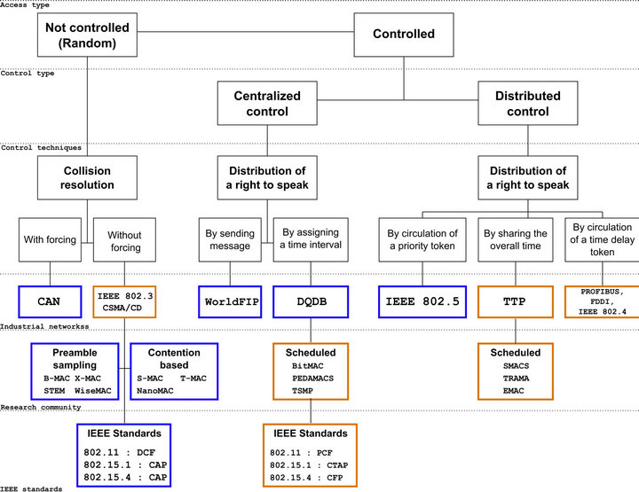
Figure 1. MAC protocols classification proposed.
In these conditions and because it is difficult to quantify the energy performances of a protocol, we propose in this paper a complementary energy analysis of different MAC protocols. Our approach is characterized by a joint approach with the addition of physic cal layer performances in the MAC layer analysis.
3. Realistic Energy Assessment Method
3.1. Method Description
All the parameters that affect energy consumption in a sensor network depends mainly on the physical layer implemented (hardware architecture, transmission power), but also on the MAC layer which defines the frames lengths necessary for dialogues between the different sensors, and in an energy point of view affect the durations of transmission and reception. However, the modelling of these parameters cannot be done while preserving a classic layering. In fact, the parameters mentioned are inter correlated and impact jointly the overall consumption. In these conditions, it is better to model the impact of these parameters by a cross-layer approach. In this way, we seek to model the increasing of the number of retransmissions due to the BER of the physical layer, i.e. the probability that a frame contains an error and requires a retransmission. In addition, we model synchronization losses at the physical layer level that cause a lengthening of the preamble field defined by the MAC layer and thus an increasing of consumption due to longer transmission durations. Finally, with MAC protocols based on a contention access, it is also necessary to model the energy consumption due to the traffic volume in the network (number of nodes). From these considerations, we present in this section, a method which allows taking into account the traffic volume on the energy consumption of a sensor. Then, we describe how to take into account the real duration to transmit a frame from the BER knowledge, and finally the synchronization losses.
3.1.1. Traffic Volume Considerations
The method used to take into account the traffic volume in the calculation of the average power consumption is based on the analysis conducted by Kleinrock & Tobagi in [15] on the latency caused by the use of CSMA/CA. In the same way as in [16], we derive this method in order to analyze the energy consumption of the 802.15.4 standard.
The aim of this method is to express analytically the proportions of time when the channel is busy because of transmissions from other sensors. Then, we derive periods of time when the channel is free of all transmissions. Knowing the proportions of these times, it is possible to express the power consumed when a sensor listens the channel while it is busy. To perform this method, we consider initially the following assumptions: a network composed of N nodes; as in [15,16] we assume that transmission attempts of each node follows a Poisson process of rate g = 1/L (with L the time interval between two transmission attempts); finally, the global rate of transmission attempts is equal to N·g.
1) Calculation of the average period when the channel is idle
The period when the channel is idle starts at the end of the frame transmission and ends at the beginning of the next transmission. Its duration can be expressed by a random variable I = Tvuln + X, with X the random time between the end of a transmission and the beginning of another, and Tvuln the vulnerable period when a node switches from the receiving state to the transmitting state after the signal strength measurement on the channel. The average duration of an idle period, can be calculated by using an exponential distribution with parameter N·g whose the cumulative distribution function is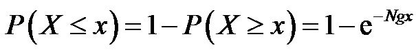 , giving an expected value equal to
 . Therefore, the average period when the channel is idle can be expressed by Equation (1):
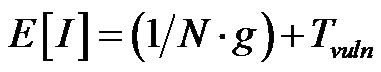 (1)
(1)
2) Calculation of the average period when the channel is busy
This period starts when a transmission starts and ends when the last frame is transmitted. Its duration can be expressed by a random variable Z = Y + TDATA with Y the random time between the first and last frame and TDATA the duration to transmit a data frame. As for the calculation of the average idle period, the average period when the channel is busy can be expressed using an exponenttial distribution with a parameter N·g leading to the Equation (2):
 (2)
(2)
3) Calculation of the average power consumed
After to have estimated the average duration of each channel state (idle and busy), it is possible to express the proportion of time b when the channel is considered busy by the Equation (3).
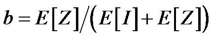 (3)
(3)
following the same approach, we know that a transmitssion will be effective only if the channel is idle, i.e. with probability (1 – b). So, the successful transmissions follow a Poisson process with a rate equal to g(1 – b), and the average occupancy of the channel due to these transmissions can be expressed simply by the duration to send a frame: E[Z1] = TDATA. The average period when the channel is idle at the transmitter level is hence equal to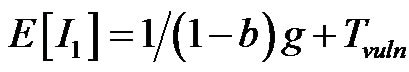 . Finally, the proportion of time b1 when a transmitter is being to transmit can be expressed by:
 (4)
(4)
3.1.2. Physical Layer Performances Considerations
The main idea in this paragraph is to take into account the physical layer performances into the energy assessment of a MAC protocol. Indeed, as noted before, the physical layer robustness against errors introduced by the propagation channel (BER), can affect the MAC layer performances and lead to frames retransmissions. Moreover, we know that a frame retransmission is required when in reception; a frame contains at least one error. The probability to have at least one error in a frame corresponds to the Frame Error Rate (FER) and depends on both the frame length fl and the Bit Error Rate (BER):
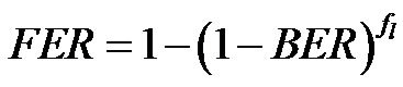 (5)
(5)
the ideal duration to transmit a frame corresponds to a successful transmission on the first try, it depends on fl the frame length and rate the data bit rate:
 (6)
(6)
the real transmission duration must take into account the additional durations due to retransmissions. It depends therefore on the FER and can be expressed by:
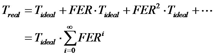 (7)
(7)
so, this is a geometrically serie which converges because . It is therefore possible to approximate it by:
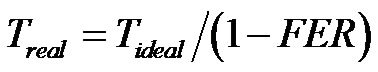 (8)
(8)
finally, the real duration to transmit or receive a frame depends on the frame length fl, the data bit rate rate and the BER:
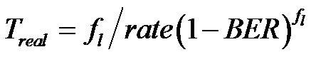 (9)
(9)
from this equation, it is hence possible to take into account in the assessment of a MAC protocol, the real durations of transmission/reception according to the BER.
3.1.3. Synchronization Losses Considerations
In practice, the clock drifts due to changes in pressure and temperature involve the use of resynchronization mechanisms between a transmitter and a receiver. These mechanisms are necessary for both the binary rhythm recuperation and the exchanges synchronization. In principle, the resynchronization is performed from the synchronization fields in the header frame. More particularly, the preamble is necessary to synchronize the information exchanges, while the synchronization word is used to recover the binary rhythm. As in [16], we assume in the worst case that if a receiver wakes up in advance and a transmitter send his frame in late, the synchronization period required to ensure the exchanges synchronization must be equal to TSync = 4θL, with θ the clock drift of the quartz and L the transmission interval. Nevertheless, if we assume that the clock drifts are uniformly distributed on [–θ;+θ], a synchronization period of TSync = 2θL is sufficient.
3.2. Protocols Definition
The aim of this section is to describe the MAC protocols chosen and which can be used by the aimed application. The application constraints lead us to study and express analytically the power consumption of three types of MAC protocols in order to compute the lifetime of a sensor using one of this protocol: an ideal protocol, which will serve as a reference maximum lifetime; the 802.15.4 standard used in industrial and home automation and which has designed particularly for low power systems; and finally, the WorldFIP protocol used princepally in industrial networks but whose the scheduling techniques implemented allow to achieve deterministic communications in order to avoid the risk of collisions.
3.2.1. Ideal Protocol
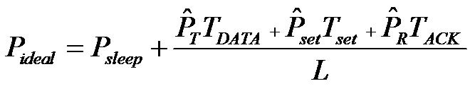
The operation of this protocol is shown in Figure 2. After the measurement of the physical quantity, the sensor decides itself to initiate a transmission to the gateway during a period TDATA. The gateway is ready to receive data and sends an acknowledgment (ACK frame) to the sensor to validate the transaction. The time interval between each transmission is denoted L. The average power consumed by a sensor can be expressed analytically by the following Equation (10).
 (10)
(10)
in this equation,  ,
, ,
, , respectively represent the power consumption increment compared to a sleep state (consuming Psleep) for transmission, reception, and a mode change. TDATA expresses the transmission or recaption duration of a data frame. Tset = TSetRx = TSetTx is the duration necessary to switch from the reception mode to the transmission mode (or inversely). Finally, TACK corresponds to the transmission or reception duration of an acknowledgment frame.
3.2.2. IEEE 802.15.4 Protocol (Zigbee based)
After the ideal protocol, we choose to assess the 802.15.4 standard. Its operation principle is illustrated in Figure 3.
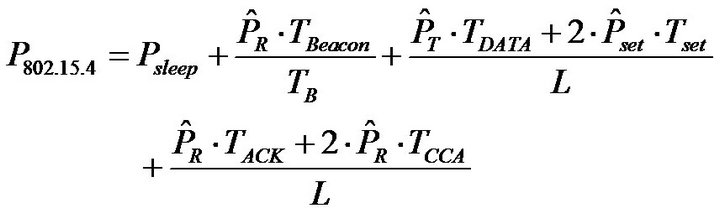
A beacon frame is sent by the gateway with a time interval TB. Each sensor listens it in order to synchronize itself with the gateway; then, they enter in a CSMA/CA slotted process to access to the channel. The Clear Channel Assessment to verify if the channel is idle, takes place over a period of 2 TCCA. The first sensor that wins the competition transmits its data and waits an acknowledgment frame. In these conditions, the average power consumed by a sensor that won the access to the channel, can be expressed by the Equation (11).
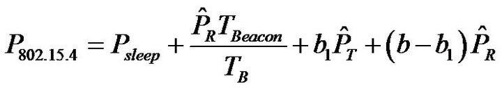
 (11)
(11)
In the same way as for the ideal protocol,  ,
, ,
, , respectively represent the power consumption increment compared to a sleep state (consuming Psleep) for transmission, reception, and a mode change. TBeacon corresponds to the transmission or reception duration of a beacon frame, TB is the interval transmission of beacons, TDATA expresses the transmission or reception duration of a data frame, Tset is the duration necessary to switch from the reception mode to the transmission mode (or inversely), TACK corresponds to the transmission or reception duration of an acknowledgment frame, and finally TCCA represents the duration for a sensor, to check if the channel is idle before attempting to transmit.
3.2.3. WorldFIP Protocol
The operation principle of this protocol is illustrated in Figure 4. The network coordinator (the gateway) serves as manager of information exchanges by using a polling
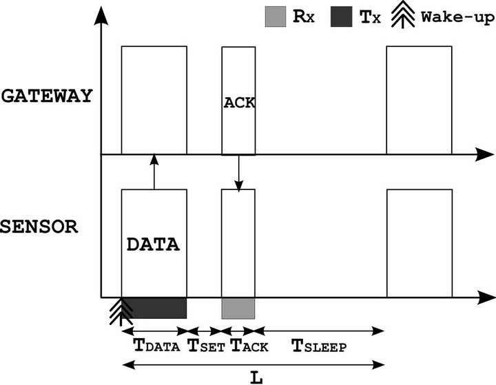
Figure 2. Operation principle of the ideal protocol.
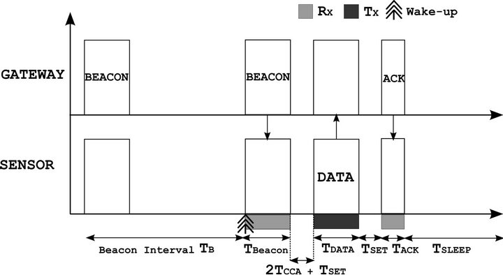
Figure 3. Principle of the 802.15.4 protocol.
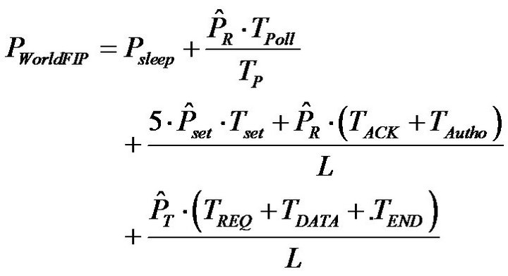
method. It interrogates each sensor one by one by sending a polling frame. If a sensor recognizes itself and has data pending, it sends a request frame in order to start a data transfer with the gateway. If the gateway is ok, it transmits an authorization frame to reserve the channel. Then, the sensor transmits its data and waits for an ACK frame to validate the transaction. The communication ends with a completion message. This exchange pattern is performed during an elementary cycle denoted TP. From this operation, the average power consumed by a sensor using this protocol can be expressed by Equation (12).
 (12)
(12)
 ,
,  ,
,  , respectively represent the power consumption increment compared to a standby state for transmission, reception, and a mode change. The time periods TACK, TAutho, TReq, TDATA, TFIN, respectively represent the durations for transmission or reception of an acknowledgment, an authorization, a request, a data and finally an end frame. TPoll corresponds to the transmission or reception duration of a polling frame. Finally, Tset corresponds to the duration necessary to switch from the reception mode to the transmission mode (or inversely).
4. Lifetime Computations and Results
The method used to estimate the performances of a MAC protocol allowed us to express analytically the average power consumed by a sensor. Then, to calculate the sensor lifetime, we use the battery model presented in [16] and the value of the CC1110 radio chip consumption [17]. The data bit rate is set arbitrarily at 250 KBps. The ideal transmission and reception durations T for each protocol are computed according to the frame lengths fl and the data bit rate considered: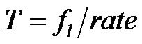 . Finally, the real durations are computed according to the Equation (10).
Each frame length is specified according to the standard and is listed in the Table 1. Moreover, to respond to the application constraints described in the section IV, we assume into the data frames a time stamping performed on 4 bytes and a data payload equal to 2 bytes.
In the following, the lifetime results are shown with three accuracy levels, in order to show the impact of the traffic volume, the physical layer performances, the synchronization losses and finally the combination of all these criteria.
4.1. First Assessment Without to Take into Account any Errors
The results in terms of lifetime for a sensor using the MAC protocols described are illustrated in Figure 5. They are obtained for a particular case when TP = TB = L, in other words when the transmission interval of a sensor is equal to the transmission interval of beacons and polling frames. Moreover, the traffic volume, the synchronization losses and the physical layer performances are not taken into account for this first result.
First, we can observe logically that the lifetimes obtained are linked to the transmission frequency. The ideal protocol gives the best efficiency with a maximum lifetime of more than 9 years when L is greater than 100 s. The performances obtained for the 802.15.4 and the WorldFIP protocol are very similar. The maximum gap between the ideal protocol and the two others is approximately equal to 3 years and it is obtained for a
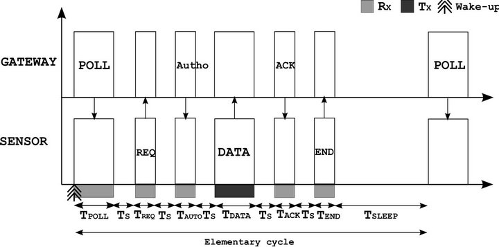
Figure 4. Principle of the WorldFIP protocol.

Table 1.Frame length (bytes) for each protocol.
transmission interval of 3 s. The 802.15.4 protocol is slightly more efficient with a maximum lifetime gain of about half a year when L is between 1 and 10 s. Finally, from 100 s, WorldFIP starts to be more efficient. It is important to note that the relatively good performances obtained are conditioned by the fact that TP = TB = L. In reality, if the transmission interval of a sensor is higher or less than the transmission interval of polling/beacon, the performances in terms of lifetime will be significantly degraded.
4.2. Second Assessment by Taking into Account the Traffic Volume in the Network
The traffic volume can only be taken into account for the 802.15.4 protocol. The impact of the traffic volume on the others protocols affects only the needs in terms of gateway computation, because the medium access mechanisms of these protocols are not based on access competition. So, from the Section 3.1.1, and by following

Figure 5. Lifetime according to the transmission interval L, when no errors are taken into account.
express the average power consumed by the Equation (13).
 (13)
(13)
with (b – b1) the time proportion where the channel is busy because of the transmission of the other sensors. The lifetimes computed from this equation are plotted in Figure 6 and for a network composed of 1, 10, 20 and 30 nodes.
Logically, we observe that if the number of nodes in the network increases, the lifetime of a particular sensor decreases. Indeed, the channel access mechanism being based on a contention access, more the number of nodes increases and more a sensor listen the channel while it is busy. More particularly, we obtain a maximum gap equal to 4 years between a network of 30 nodes and a network without any traffic, when the transmission interval L = 10 s. In addition, we can note that more the number of
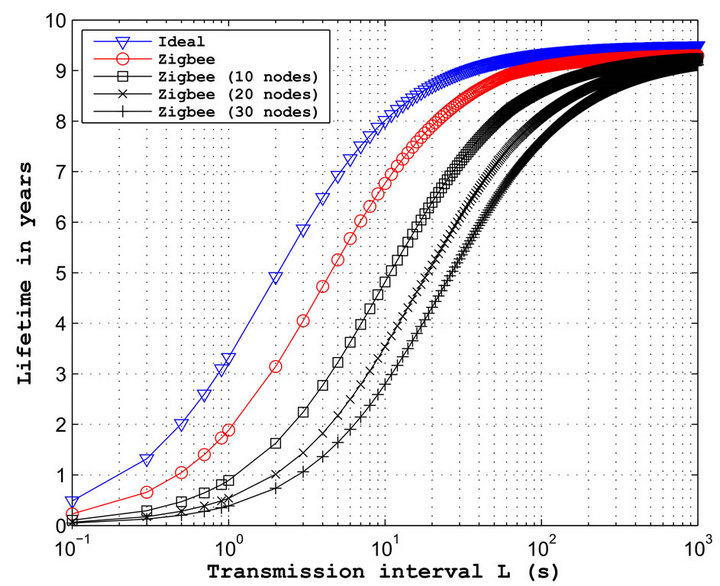
Figure 6. Lifetime according to the transmission interval L, with traffic volume taken into account.
nodes increases and more it is essential to increase the transmission interval to obtain the same performances as the ideal case. Indeed, it is necessary to have transmission intervals more important in order to avoid the transmission or the carrier sensing of two nodes simultaneously. However, for significant transmission intervals, the lifetimes obtained are similar whatever the number of nodes. In this case, the sleep duration dominates the global consumption.
This illustration of lifetime degradation is important to consider for this MAC protocol type. The performances obtained underscore the interest of a deterministic MAC protocol whose performances are not dependent on the traffic volume.
4.3. Third Assessment by Taking into Account the Physical Layer Performances
The lifetimes of a sensor obtained by taking into consideration the physical layer, and hence the real time of frame transmissions, are plotted in Figure 7.
The curves in red and blue respectively represent the lifetimes when BER = 0 for the WorldFIP and the 802.15.4 protocols. For the both protocols, the performances obtained when the BER = 10–3, are very close to the performances obtained when the BER is null. For this level of errors, the number of retransmissions is quite low because the frame lengths of each protocol are quite low. However, if the BER ≥ 10–3, the lifetimes obtained decrease significantly. We can note a lifetime reduction of 2 years for WorldFIP and 3 years for 802.15.4. In this case, the BER involves important retransmissions. Finally, the performances displayed by the protocol WorldFIP are much better, because the frames lengths implemented in this protocol are lower than those implemented in the 802.15.4 standard.
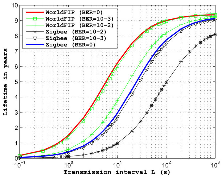
Figure 7. Lifetime according to the transmission interval L and the BER.
The physical layer consideration at the MAC layer level is interesting in two aspects. It allows seeing the impact of physical layer performances on a MAC protocol, but it allows also showing the importance of the frame lengths on the average lifetime of a sensor.
4.4. Fourth Assessment by Taking into Account the Synchronization Losses
As noted before, a receiver must be awakened in advance to receive beacon or polling frames and to be sure to not miss the transmission according to the importance of clock drifts. This period of time required for the synchronization exchange is proportional to the time since the last resynchronization. By considering a clock resynchronization at each beacon/polling frame reception, the period needed to compensate clock drifts is equal to TSync = 2θL, with L = TB = TP. Whatever the protocol, the additional energy required to compensate the clock drifts is hence equal to 2.θ.PR. The lifetimes obtained in these conditions are plotted in Figure 8.
There is very clear that the performances of each protocol are degraded when the transmission interval is large. When L ≥ 10 s, we can observe a reduction of the lifetime of more than a year. In contrast, the performances observed when L ≤ 10 s are very similar to the performances obtained without any consideration of errors. In this case, the transmission frequency is quite high, leading in quite low clock drifts and thus to an energy consumption overhead negligible.
4.5. Last Assessment with the Combination of All Criteria
Finally, the lifetimes obtained according to the transmission interval are represented in Figure 9 for a network composed of 30 nodes, and by considering the synchro
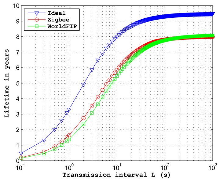
Figure 8. Lifetime with synchronization losses taken into account.
nization losses and a BER = 10–3.
The results clearly show the impact of the transmission conditions on the energy performances. There is very clear that the 802.15.4 protocol is less efficient. There is a difference of nearly six years for a transmission interval L = 10 s between this protocol and the ideal protocol. For transmission intervals greater (L ≥ 100 s), the difference is more than a year. The WorldFIP protocol shows much better performances.
For L = 10 s, the difference with the ideal protocol is only equal to three years. For transmission intervals greater, the performances obtained are very close to performances obtained with the 802.15.4 protocol. Nevertheless, it is necessary to be careful by interpreting the results of the WorldFIP protocol. Indeed, the performances obtained are mainly due to the low frame lengths specified by the protocol. However, if these lengths are valid for a wired transmission medium, it is different for a wireless medium. The frames headers necessary to recover the binary rhythm are lower because the errors introduced by a wired transmission medium are less numerous than in the case of a wireless transmission medium. To conclude, the results presented underscore therefore the frame lengths importance compared to the exchange scheme to obtain energy efficient communications.
5. MAC Protocol Proposal
5.1. Application Description
The aimed application is a building monitoring system based on a WSN. The system must perform in situ measurements (physical quantities and building use) in order to assess in a qualitative way the building performances. These measurements can allow performing annual or statistics reports in order to know for example the average
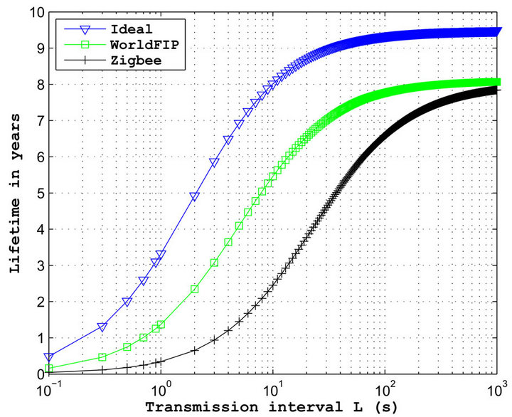
Figure 9. Lifetime according to the transmission interval L with all errors taken into account.
noise level with windows closed and ventilation system in operation or the number of hours of use of electric lighting.
The aim of such system is to perform a long term study with a fine temporal resolution. In these conditions, the WSN autonomy must be of several years. The radio frequency band chosen are the 433 and 868 MHz band (ISM bands in France) for their transmission range and energy efficiency properties. Moreover, we assume in this paper, a 1-hop centralized network.
The network architecture (Figure 10) is hence composed of 3 elements: sensors, gateways and a server.
• The sensors must operate on batteries. We distinguish two types of sensors: periodic and event sensors. The role of periodic sensors is to measure periodically some physical quantities (light, temperature, humidity) whereas the role of event sensors is to assess the building use by measuring the occupants’ behaviour (presence/absence, state of opens).
• The gateway is assumed connected to the mains. His aim is to manage and collects the data from 2 or 3 rooms (or a transmission range of 25/30 meters).
• The server is used as a database for the data storage, and it must be accessible by a web navigator.
The transmissions between sensors and gateways are performed in a wireless medium and the communications between gateways and the server is performed through a wired connexion using the Ethernet protocol. The OSI model for this network is hence reduced in three layers, the application layer, the MAC layer and the physical layer. The cost constraints involve a network size of 200 sensors at maximum, and the needs fixe the sensors number per room to 10. Finally, the needs at the level of the data analyses involve a time stamping to perform detailed reports.

Figure 10. Building monitoring system based on a WSN.
5.2. MAC Protocol Proposal
The aim of this last part concerns the proposal of a MAC protocol that takes into account all the constraints of the aimed application described in the previous section. This protocol must allows to manage the periodic and non-periodic communications while remaining enough flexible and scalable to facilitate the integration of new sensors types in the network. Moreover, the protocol must be energy efficient to allow the network deployment during several years.
The results obtained in the previous cross-layer energy analysis allow us to highlight the impact of the frames lengths in the final performances of a protocol. This impact has been particularly emphasized with the WorldFIP protocol, which despite an important number of exchanges, provides good performances due to its small frames lengths. To obtain an energy efficient MAC protocol, there is therefore essential to minimize jointly the frames lengths and the exchanges number.
The idea adopted and represented in Figure 11 is based on a static allocation of the channel centrally managed by a coordinator according to a bandwidth shared in time.
During a primary cycle, the gateway polls each sensor one by one and asks them to transmit their data. This time period is dedicated to the periodic traffic manage ment. This traffic concerns all periodic sensors (temperature, humidity, light ...). The secondary cycle is dedicated to the non-periodic traffic management and concerns the event sensors (presence detectors, state of the doors ...). The initial idea is to allocate a specific time interval for the management of this traffic. At the sight of application requirements and specifications time, the proposed solution is similar to the periodic traffic management. Each periodic sensor is asked one by one to see if it has detected an event. This detectors sampling must be performed with a correct frequency to not miss any event. Its efficiency depends on the number of periodic sensors and on time allocated for each to perform a valid data transaction. In order to ensure fair and bounded access for each sensor and detector, the primary and secondary cycle’s durations are bounded. After the polling of all sensors and detectors performed, the remaining time is allocated to the network management. This time period allows taking into account the introduction of a new sensor in the area covered by the gateway or even the introduction of a maintenance computer.
The construction of the scheduling is based on an offline algorithm and the temporal resolution depends on the sensors number managed by the gateway. The primary or secondary cycle duration corresponds to the sensors number multiplied by the duration of an information exchange. In this way, the management method used is deterministic. The collision risk is avoided because a time slot is allocated for each sensor. In addition, in case of failure, a return path is possible during the network management. To complete the construction of the temporal scheduling, the assignment and the priority messages arbitration can be performed simply by taking into account the firing sensors order during an initialization phase.
5.3. Exchange Scheme Definition
The exchange scheme for a communication between the gateway and a sensor is shown in Figure 12.
This exchange scheme is minimal, it is a simple periodic polling mechanism performed by the transmission of polling frames (POLL) which allow to initiate a com-
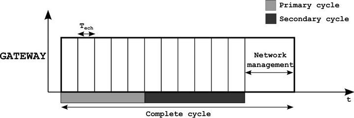
Figure 11. Time sharing of bandwidth.
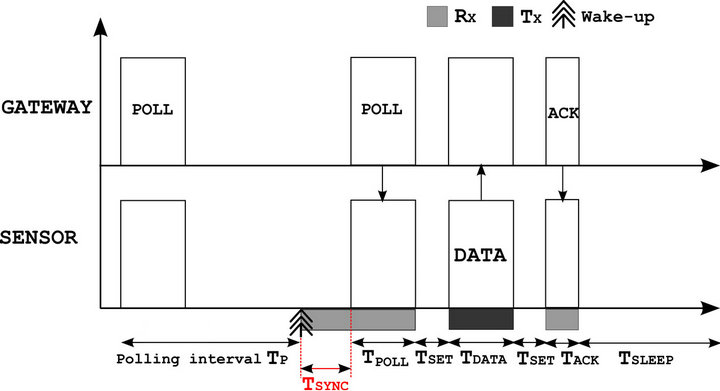
Figure 12. Exchange scheme of the solution.
munication. Once the data transmitted by the sensor, an acknowledgment frame is sent by the gateway to valid the transaction. From this principle, we can express the average power consumed by Equation (14).
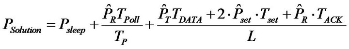
(14)
the time periods TACK, TPOLL, respectively represent the times to transmit or receive a acknowledgment and a polling frame. Tset corresponds to the duration necessary to switch from the reception mode to the transmission mode (or inversely). Finally, the transmission interval of polling frames is denoted TP. This interval TP is always equal to the transmission interval L. In other words, at each sensor wake-up by the polling frames, a transmission of one information is guaranteed. The synchronization period Tsync is not expressed in the equation (14). We show later that the time required to compensate the clock drifts is taken into account through the polling frame, so through the duration TPOLL.
5.4. Definition of Frame Formats
The frame formats must be compliant with the application requirements on one hand and with the energy constraints on the other hand. The solution chosen to comply the application requirements is based on the definition of an additional field indicating the frame type and the service requested. The answer to the energy efficiency question is based on the frame lengths reduction. The aim is both to minimize the sensor consumption in transmission mode by reducing the data frame length and in the same way, the sensor consumption in reception, by reducing the polling frame length.
1) Polling frame
The final format chosen for a polling frame is shown in Figure 13.
A preamble is required for the different synchronization levels in reception. The preamble chosen is composed of two parts. One part is dedicated to the clock drifts compensation in order to synchronize communications between the gateway and a sensor. This is the field CDC. Referring to the section 3.1.3 on synchronization losses in the energy analysis, we know that it is necessary to compensate the drifts due to the quartz inaccuracies, in order to have a good exchanges synchronization when one of the two communicating entities is in advance or in late to its schedule. We know also that in the worst case, the synchronization period necessary is TSync = 4θL. To avoid the synchronization losses, the first part of the preamble is hence used to compensate the clock drifts with a length fixed at 4θL. In practice, it is necessary to centre the preamble at the moment of the receiver awakening by aiming a transmission to TX = L – CDC/2.
The other part of the preamble, the synchronization word, is necessary for carrier and binary rhythm recovery in order to demodulate the data correctly in reception. His length is determined according to the hardware architecture used. In practice, the carrier and binary rhythm recovery is often performed by a digital PLL. It is hence necessary to know the PLL acquisition time. This is generally difficult to quantify because it depends on the initial errors on the phase and frequency and on the pattern chosen for the synchronization word. Based on studies in [18,19], we admit in this paper, the use of a digital PLL whose performances in terms of acquisition time requires the use of a sync word equal to 2 bytes.
A frame type field and an ID field respectively allow to identify the service type requested and to indicate the
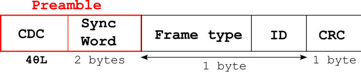
Figure 13. Polling frame format used by the gateway.
message receiver. These two fields are combined in a one byte field, allowing the management of more than 200 sensors with more than a dozen frame types.
A CRC field is required to check data integrity in reception. Its efficiency depends on both the polynomial length and the data field length. Based on the study in [20] and compared to the data payload length necessary in our application, a CRC of one byte is sufficient.
The special feature of this frame type concerns the preamble. It is adaptive to compensate the clock drifts and to ensure a good communications synchronization between the gateway and the sensors. The total polling frame length depends on the transmission frequency 1/L but contains a fixed part always equal to 2 bytes with the synchronization word.
2) Data and acknowledgement frames
The structure of a data frame is shown in Figure 14.
In the case of a data frame, the preamble is not adaptive because the time between the reception of the polling frame and the transmission of the data frame is enough short to maintain the synchronization. In addition, to reduce the data frame length, we consider that a timestamp field is not necessary. In reality, with the desired accuracy level, the arrival time of messages at the gateway level is sufficient to timestamp data. In these conditions, the total data frame length is set to 6 bytes.
An acknowledgment frame has the same structure as the data frame. But, its frame type field is modified and the data field is removed. The final ACK frame length is hence equal to 4 bytes.
6. Proposed Solution Assessment
The aim of this part is to assess our proposal compared to the other MAC protocols. For this, we use the same analytical description that before.
6.1. First Assessment Without to Take into Account the Physical Layer Performances
In this section, the physical layer performances are not taken into account but the traffic volume (N = 30 nodes) and the synchronization losses are included in the assessment. Moreover, the transmission interval of beacons/polling frames is equal to the transmission interval of the sensors: TB = TP = L.
Figure 15 represents the lifetimes obtained according to the transmission interval L.
First, we observe that the ideal protocol is the most efficient, but our proposal MAC protocol is much better than 802.15.4 protocols and WorldFIP whatever the transmission interval L. For high transmission frequencies, our proposal provides performances close to the ideal protocol. Then, for L = 10 s, we get a lifetime of 7 years against 2.5 years for 802.15.4 and 5.5 years for

Figure 14. Data frame format.
WorldFIP. Finally, for high transmission intervals when L ≥ 100 s, the lifetimes obtained are very similar to the other protocols.
6.2. Second Assessment by Taking into Account the Physical Layer Performances
The results of the previous section seem encouraging, however the physical layer performances are not considered. It is therefore essential to visualize the physical layer impact on the performances of the proposed protocol. Results are plotted in Figure 16 for a BER = 10–3.
We can observe two behaviours on the sensor lifetime which use our protocol. First, when the transmission interval L is quite high, the lifetime obtained is similar to the previous results (Figure 15). In this configuration, the preamble of clock drift compensation CDC has a short length because L is small. In this case, the real time to transmit a polling frame is similar to the ideal time, i.e. without retransmission. From L = 15 s, the lifetime starts to fall. In fact, from this transmission interval, the synchronization losses between the gateway and a particular sensor can become too high resulting in a preamble CDC also too large. Thus, the number of retransmissions for a BER = 10–3 becomes itself too important, impacting directly the sensor lifetime. These results show again the importance to take into account the physical layer performances in the assessment of a MAC protocol.
6.3. Solution Modification and Assessment
To reduce the CDC preamble length, it is necessary to reduce the synchronization losses by using periodic resynchronizations through polling frames. So, for high transmission intervals, when the clock drifts are low, the polling frames can be sent at the same rate as the sensor transmission interval: TP = L. Then, for larger transmission intervals, the transmission interval of polling frames must be fixed to periodically resynchronize a sensor with its gateway. In this way, the CDC preamble length is reduced.
In these conditions, for a BER = 10–3, the transmission interval of polling frames is set at TP = L for 0, 1 s ≤ L ≤ 15 s, and then from L ≥ 15 s, the interval is set at TP = 15 s. The results are shown in Figure 17.
Despite the addition of an extra consumption caused by the periodic transmission of polling frames to avoid too long preambles, the observed results are interesting. Through this periodic resynchronization, performances
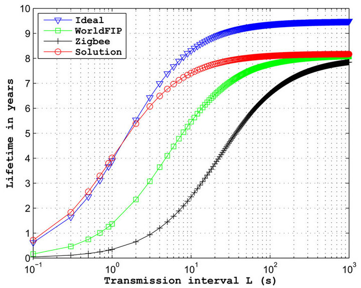
Figure 15. Lifetime according to the transmission interval L of our proposal, when the physical layer performances are not taken into account.
obtained are very close to the ideal case (Figure 15). Nevertheless, the lifetime observed is slightly less efficient. The sensor lifetime loses nearly 0.5 year when the transmission interval L ≥ 15 s. However, the results are good compared to the 802.15.4 and the WorldFIP protocol. Our proposal is more efficient than 802.15.4 protocol up to L = 300 s. After, the 802.15.4 protocol is slightly better. The lifetime gain can even reach up to 4 years when L = 10 s. Compared to the WorldFIP protocol, the performances are less pronounced but still remain very reasonable. Up to L = 40 s, our MAC protocol is the most efficient, then there is a gap of nearly 0.5 year. Moreover, it is important to remember that the 802.15.4 and WorldFIP protocols performances are generally less efficient than those presented in this paper. As noted before, the WorldFIP protocol is originally not designed to comply the wireless transmission requirements. Thus, the synchronization preamble of this protocol is certainly not suitable.
7. Conclusions
In this paper, we have shown that the modelling of the parameters affecting the energy consumption cannot be done while preserving a classic layering. From this postulate, we have presented a realistic cross-layer methodology to assess the real performances of a MAC protocol, by taking into account the physical layer performances but also the synchronization losses and the traffic volume in the network. After the assessment of three protocols adapted to our application, we have demonstrated the importance to reduce jointly the frames lengths and the exchanges number. This analysis led us to a MAC protocol proposal which complies all the aimed application constraints. The performances obtained in terms of lifetime are good and in the most cases better than those obtained with the 802.15.4 protocol.

Figure 16. Lifetime according to the transmission interval L of our proposal, when the BER = 10−3.
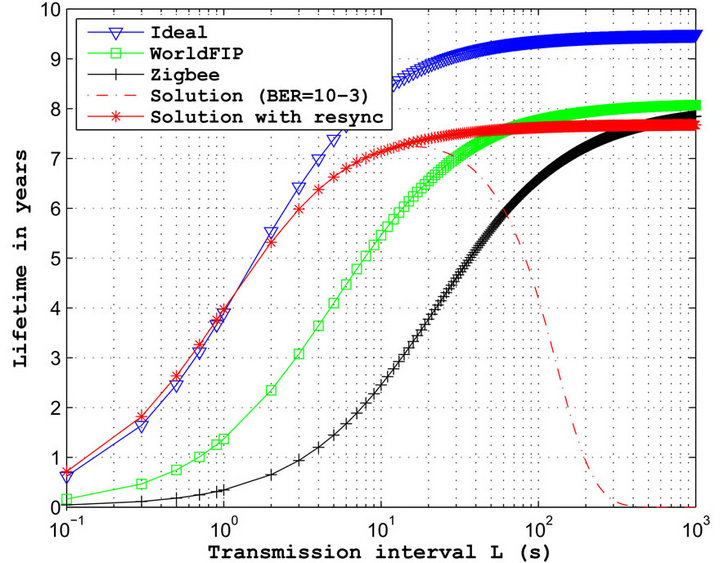
Figure 17. Lifetime according to the transmission interval L of our proposal, when the BER = 10−3 and by modifying the synchronization period.
However, it is important to note that in the case of a centralized protocol (in our case with the gateway), the performances are conditioned by the gateway capacities (power supply and computation). In other words, the energy efficiency of our protocol is based on a single entity, the coordinator of exchanges. In case of gateway failure, the network operation can be interrupted. It is therefore essential to provide a battery backup to avoid a power supply problem.
Moreover, the efficiency of our proposal is based partly on the adaptive preamble definition that ensures a good timing of communications. In the case of large transmission intervals, the preamble length can be important, so a periodic resynchronization is required. Other solutions can be used to minimize the preamble length. It is possible for example to use mechanisms in order to learn the clock drifts, but this kind of solution is not treated in this paper.
Finally, it is important to note that the efficiency weight of our proposal is based on the network initialization and on the time slots allocation while maintaining a good flexibility for the integration of new sensors types. This initialization phase is therefore essential to ensure good performances.
REFERENCES
- A. Mainwaring, D. Culler, J. Polastre, R. Szewczyk and J. Anderson, “Wireless Sensor Networks for Habitat Monitoring,” Proceedings of the 1st ACM International Workshop on Wireless Sensor Networks and Applications, New York, September 2002, pp. 88-97. doi:10.1145/570738.570751
- S. Lin, J. Zhang, G. Zhou, L. Gu, J. Stankovic and T. He, “ATPC: Adaptive Transmission Power Control for Wireless Sensor Networks,” Proceedings of the 4th International Conference on Embedded Networked Sensor Systems, New York, November 2006, pp. 223-236. doi:10.1145/1182807.1182830
- D. Dessales, A.-M. Poussard, N. Richard, R. Vauzelle, C. Martinsons and F. Gaudaire, “Transmission Power Adaptation According to the Message Length for Wireless Sensor Networks,” IEEE 22nd International Symposium on Personal Indoor and Mobile Radio Communications (PIMRC 2011), Toronto, 11-14 September 2011, pp. 46- 50. doi:10.1109/PIMRC.2011.6140005
- K. Langendoen and G. Halkes, “Energy-Efficient Medium Access Control,” In: R. Zurawski and ISA Corporation, Eds., Embedded Systems Handbook, CRC Press, San Francisco, 2005, pp. 256-287.
- E. Callaway, “Wireless Sensor Networks: Architectures and Protocols,” Auerbach Publications, Boca Raton, 2004.
- T. Melodia, M. Vuran and D. Pompili, “The State of the Art in Cross-Layer Design for Wireless Sensor Networks,” In: M. Cesana and L. Fratta, Eds., Wireless Systems and Network Architectures in Next Generation Internet, Vol. 3883, Springer, Berlin, 2006, pp. 78-92. doi:10.1007/11750673_7
- F. Vasques and G. Juanole, “Fieldbus MAC Mechanisms for Hard Real Time Data Communication Support,” Proceedings of International Conference on Open Bus Systems, November, 1993, pp. 225-232.
- W. Ye, J. Heidemann and D. Estrin, “An Energy-Efficient MAC Protocol for Wireless Sensor Networks,” Proceedings of 21st Annual Joint Conference of the IEEE Computer and Communications Societies, Vol. 3, 2002, pp. 1567-1576. doi:10.1109/INFCOM.2002.1019408
- T. Van Dam and K. Langendoen, “An Adaptive EnergyEfficient MAC Protocol for Wireless Sensor Networks,” Proceedings of the 1st International Conference on Embedded Networked Sensor Systems, ACM, New York, 2003, pp. 171-180. doi:10.1145/958491.958512
- A. Bachir, D. Barthel, M. Heusse, M. Heusse and A. Duda, “Micro-Frame Preamble MAC for Multihop Wireless Sensor Networks,” IEEE International Conference on Communications (ICC’06), Vol. 7, 2006, pp. 3365-3370. doi:10.1109/ICC.2006.255236
- A. El-Hoiydi and J. Decotignie, “WiseMAC: An Ultra Low Power MAC Protocol for the Downlink of Infrastructure Wireless Sensor Networks,” Proceedings of the 9th International Symposium on Computers and Communications (ISCC 2004), Vol. 1, 2004, pp. 244-251. doi:10.1109/ISCC.2004.1358412
- “IEEE Standard for Information Technology-Telecommunications and Information Exchange between Systems, Local and Metropolitan Area Networks, Specific Requirements. Part 11: Wireless LAN Medium Access Control (MAC) and Physical Layer (PHY) Specifications,” IEEE Std. 802.11-2007, Revision of IEEE Std 802.11-1999, 2007.
- “IEEE Standard for Information Technology-Telecommunications and Information Exchange between Systems, Local and Metropolitan Area Networks, Specific Requirements. Part 15.3: Wireless Medium Access Control (MAC) and Physical Layer (PHY) Specifications for High Rate Wireless Personal Area Networks (WPANs) Amendment 1: MAC Sublayer,” IEEE Std. 802.15.3b- 2005, Revision of IEEE Std. 802.15.3-2003, 2005.
- “IEEE Standard for Information Technology-Telecommunications and Information Exchange between Systems, Local and Metropolitan Area Networks, Specific Requirements. Part 15.4: Wireless Medium Access Control (MAC) and Physical Layer (PHY) Specifications for Low-Rate Wireless Personal Area Networks (WPANs),” IEEE Std 802.15.4-2006, Revision of IEEE Std 802.15.4- 2003, 2006.
- L. Kleinrock and F. Tobagi, “Packet Switching in Radio Channels: Part I—Carrier Sense Multiple-Access Modes and Their Throughput-Delay Characteristics,” IEEE Transactions on Communications, Vol. 23, No. 12, 1975, pp. 1400-1416. doi:10.1109/TCOM.1975.1092768
- A. El-Hoiydi, “Spatial TDMA and CSMA with Preamble Sampling for Low Power Ad Hoc Wireless Sensor Networks,” IEEE Proceedings of 7th International Symposium on Computers and Communications (ISCC 2002), Italy, July 2002, pp. 685-692. doi:10.1109/ISCC.2002.1021748
- “CC1110 Datasheet,” Texas Instruments. http://www.ti.com/lit/ds/symlink/cc1110f32.pdf
- D. Paranchych and N. Beaulieu, “Performance of a Digital Symbol Synchronizer in Cochannel Interference and Noise,” IEEE Transactions on Communications, Vol. 48, No. 11, 2000, pp. 1945-1954. doi ; 10.1109/26.886500
- H. Brugel and P. Driessen, “Variable Bandwidth DPLL Bit Synchronizer with Rapid Acquisition Implemented as a Finite State Machine,” IEEE Transactions on Communications, Vol. 42, No. 9, 1994. pp. 2751-2759. doi:10.1109/26.317416
- P. Koopman and T. Chakravarty, “Cyclic Redundancy Code (CRC) Polynomial Selection for Embedded Networks,” IEEE International Conference on Dependable Systems and Networks, Italy, 28 June-1 July 2004, pp. 145-154. doi:10.1109/DSN.2004.1311885