Wireless Sensor Network
Vol.5 No.4(2013), Article ID:30906,9 pages DOI:10.4236/wsn.2013.54009
MED-BS Clustering Algorithm for the Small-Scale Wireless Sensor Networks
National Engineering School of Sfax, Higher Institute of Technological Studies of Gabès, Gabès, Tunisia
Email: benfradj_awatef@yahoo.fr, nejah.nasri@isecs.rnu.tn, med.farah@yahoo.fr, abdennaceur.kachouri@enis.rnu.tn
Copyright © 2013 Awatef Ben Fradj Guiloufi. This is an open access article distributed under the Creative Commons Attribution License, which permits unrestricted use, distribution, and reproduction in any medium, provided the original work is properly cited.
Received January 12, 2013; revised February 11, 2013; accepted February 25, 2013
Keywords: Wireless Sensor Networks (WSNs); Clustering; Clusterhead
ABSTRACT
With the spectacular progress of technology, we have witnessed the appearance of wireless sensor networks (WSNs) in several fields. In a hospital for example, each patient will be provided with one or more wireless sensors that gather his physiological data and send them towards a base station to treat them on behalf of the clinicians. The WSNs can be integrated on a building surface to supervise the state of the structure at the time of a destroying event such as an earthquake or an explosion. In this paper, we presented a Mobility-Energy-Degree-Distance to the Base Station (MED-BS) Clustering Algorithm for the small-scale wireless Sensor Networks. A node with lower mobility, higher residual energy, higher degree and closer to the base station is more likely elected as a clusterhead. The members of each cluster communicate directly with their ClusterHeads (CHs) and each ClusterHead aggregates the received messages and transmits them directly to the base station. The principal goal of our algorithm is to reduce the energy consumption and to balance the energy load among all nodes. In order to ensure the reliability of MED-BS, we compared it with the LEACH (Low Energy Adaptive Clustering Hierarchy) clustering algorithm. Simulation results prove that MED-BS improves the energy consumption efficiency and constructs a stable structure which can support new sensors without returning to the clusters reconstruction phase.
1. Introduction
During recent years, we have seen a miniaturization brings technology. This aptitude for the miniaturization brought a new generation of telecommunication networks which presents important challenges. The Wireless Sensor Networks are one of the technologies aiming at solving the problems of this new telecommunication and computer age [1].
The WSNs are composed of a large number of nodes communicating between them and distributed on a given geographic zone to measure a physical quantity or to supervise an event (temperature, pressure, earthquake···) ([2-5]).
The WSNs architecture breaks up into three underlayers: a sensor network which is composed of the information received from the external world, the clusterheads witch carried out the complex tasks of signal treatment, and a base station which received the information on behalf of the clusterheads ([5-7]).
The WSNs are particular networks, having different characteristics from the wired networks (absence of infrastructure, resource’s constraints, heterogeneity and dynamics structure). So, it was necessary to think of an auto-organized virtual topology which should be adaptive and effective in energy ([8,9]).
To conceive such topology, several solutions were suggested in the literature like the clustering, the heterogeneous networks and the dorsal.
In this paper, we proposed a clustering algorithm adopted with the small-scale Wireless Sensor Networks which goal is the minimization of the energy consumption by taking on account the patient’s mobility.
2. Previous Work
In this section, we will classify the clustering algorithms according to whether the deployed nodes are homogeneous (have the same features) or heterogeneous.
2.1. Clustering Algorithm: Heterogeneous Nodes
Heterogeneous network is a network where certain nodes have more raised capacities (processor, capacity for treatment, power of transmission, band-width, power of energy,···) than others. The use of heterogeneous networks can triple the delivery average rate and offer a network lifetime five times larger than the homogeneous networks [10].
Several algorithms of heterogeneous networks were invoked in the literature such as [11], where the authors propose an algorithm called GS3. It is an evolutionary and distributed algorithm intended for the wireless networking. The network is covered with a virtual hexagonal structure, the heterogeneous nodes choose the clusterheads of the hexagonal cells’ neighbors, the heterogeneous nodes which were not selected as clusterheads connect the cells as members. The same procedure is repeated to the total cover of the network. GS3 attaches a great importance to the geographical ray of the cluster, which influences according to Zhang and Arora on dissipated energy (network lifetime), on the effectiveness of the functions of local coordination and finally on the evolutionarily and availability of a network. However, topological changes of super-nodes need a total reorganization of all the structure. Moreover, GS3 requires that the super-nodes be equipped with directional antennas to enable them to reposition itself in the center of their hexagonal cell, which makes it ineffective for the majority of the classical applications.
The authors introduce another algorithm of the heterogeneous nodes in [12], called LBC (Load-balanced clustering). LBC uses many Gateways, which has a more important energy capacity: each gateway is responsible for managing the totality of its group, to correlate the data and to organize the sensors in a cluster. Each sensor belongs to one and only one Gateway, and this Gateway is its only means to communicate with the base station. In order to ensure the balance load, the super-nodes must have all information about the network and decide the optimal cluster size, this requires much information collection time. Added to that, the algorithm requires that each node is equipped with a system of localization such as a GPS (Global Positioning System.) which proves to be expensive. Moreover, one topology change requires a total rebuilding of topology. An improvement of this algorithm was proposed in [13].
Another algorithm was proposed in [14], its aims is to balance the load between nodes by using heterogeneous nodes. The heterogeneous nodes are selected like stations of data collection, which improve by consequence the lifetime of the network. To guarantee the stability of the structure, this algorithm offers a maintenance procedure in which, a topological change is treated locally. Nevertheless, the algorithm generates a high number of clusters. That impacts the cost of communication inter-cluster and the delivery period.
Others authors proposed the DEEC (Distributed Energy Efficient Clustering) [15] algorithm, the clusterheads election criterion was probabilistic and based on the waste heat of the nodes as well as the average energy of the network. If the probability of a node is higher than a certain threshold, then, it can become a clusterhead.
Admittedly, this algorithm is effective and makes nodes share energy consumption between, but the enormous exchange of the control messages can involve a performance degradation of the structure.
MDC/PEQ (Mobile data collector/PEQ) [16] was proposed like an algorithm of data collection intended to solve the critical time applications. This algorithm aims to decrease the load and to reduce energy consumption. With the super mobile nodes deployed in the interest zone, static nodes were employed to guarantee a fixed way between nodes and base station. The purpose of this procedure is the transmission of the urgent data to the destination.
Another example of the clustering heterogeneous nodes’ algorithm is found in [17]. The clusterheads election criterion is probabilistic and depends on the waste heat of nodes. In addition, this algorithm does not consider nodes mobility.
Cheick Tidjane KONE introduced into [18] new communication architecture for great dimensional sensor networks. He worked on heterogeneous structures based on the clustering to improve the performances of the network and to ease its management and its extensibility. The built clusters were limited of many hops in order to decrease the number of retransmission and the latency. KONE showed that the use of the multichannel strategy improves the network performances in terms of load and energy consumption.
2.2. Clustering Algorithm: Homogeneous Nodes
Several researchers such as [19] choose these types of algorithms. The election of the clusterheads in LCA (Linked Cluster Algorithm) is based on the ID of nodes. The communication between the clusters is carried out using the selected gateways according to their sites. The structure built by LCA allows a communication between the nodes, diffusion of the messages and on avoidance of hidden problem of station. Moreover, LCA is robust against the breakdowns and topology changes.
In 1995, the HCC (Highest Connectivity Cluster) [20] algorithm was proposed, the choice of clusterheads was based on the nodes’ degree (number of the neighbors). Topology would be configured dynamically to support the mobility of nodes. Gerla and Tsai compared the algorithms LCA and HCC and showed that the first preserved the stability of structure.
In 2000, Amis and al. introduced the algorithm max-Min d-cluster [21]. The clusterheads election proceeds in two stages: a first stage made up of D-turns where the nodes choose the highest ID like winner value (WINNER), and a second whose selected values are those of weakest IDs. The goal of this algorithm is the minimization of the load, minimization of the number of clusterheads formed as well as the stability of the network. However, the knowledge of the neighborhood with D-hops requires enormous exchanges of messages and leads to a considerable latency.
Another example of clustering is found in [22], it is the most popular algorithm. LEACH chooses by chance the clusterheads for one time according to a policy called “Round Robin”. The communication intra-cluster as well as the communication between the clusterheads and the base station is carried out in 1-hop. The principal goal of LEACH is the balance of energy dissipation between sensors. Nevertheless, the election procedure (random) can lead clusterheads to have a weak energy reserve, which can affect the data transmission and can lead to a reconfiguration of the built structure.
Several improvements were made to LEACH such as LEACH-C [23] (LEACH-Centralized), which implies the remaining energy of nodes in the criterion of clusterheads election. This algorithm was called centralized LEACH because the procedure of clustering is controlled by the base station. A second example is M-LEACH [23] algorithm (Multi-hops LEACH). Contrary to LEACH, the connection intra-cluster is multi-hops, these involve a stability of the structure by reducing clusterheads dissipated energy. LEACH-F (LEACH with Fixed Cluster) is another algorithm based on LEACH. This algorithm proposes that the formed clusters are fixed, and the nodes’ mobility is not considered.
In 2002, Chatter and al. introduced an algorithm based on the principle of LCA called WCA (weighted Clustering Algorithm) [24]. The clusterheads selection criterion depends on their degrees of connectivity, their powers of transmission, their mobility and their energy reserves. The authors still require that the dominant nodes have to be in the center of their cells and that the nodes’ number is limited in each zone, which poses a problem with the dynamic structures.
Mitton and al. proposed a clustering algorithm in [25] whose clusterheads election was based on K-density metric. The k-density of a node east defines as the relationship between the bonds and the number of node in a K-neighbourhood. This algorithm offers the maintenance policy ensuring more stability of the structure by choosing the same nodes each time if that is possible.
HEED (Hybrid Energy-Efficient Distributed) [26] algorithm is developed in 2004 by Y. Ossama and S. Fahmy. The choice of the clusterheads depends on their degrees of connectivity and their reserves on energy. The principal goal of HEED is to balance energy consumption between nodes.
DEBC [27] (Distributed Energy Balance Clustering) is an algorithm of clustering invented by Duan and Fun in 2007, the clusterheads election criterion is probabilistic and depends on the nodes remaining energy. This algorithm is supposed to be complex because of enormous number of transmitted messages which makes it more effective for the small networks.
In 2008, Yu and al. introduced the EEDMC [28] (Energy-Efficient Distributed Multi-level Clustering) algorithm whose goal was the minimization and the balancing of the energy consumption. The node weight is defined as being the quotient between its average residual energy and the medium residual energy of its neighbors. A multi-hops communication is supposed between the clusterheads and only one clusterhead is selected for the communication with the base station. The simulation results show that EEDMC is effective and allows increase the lifetime of the network.
3. Contribution
The sensors networks are used for vital and crucial applications (monitoring of habitat, detection of earthquake, military monitoring, ···). For this reason, reliability represents a very important challenge ([5,6], [29,30]). In addition, energy consumption (lifetime of network) presents the most important metric in the performance evaluation of network [1]. Indeed, the lifetime is regarded as a fundamental factor in the context of availability in the WSN [31]. This parameter poses energy safeguarding problems particularly if the application must work a long time. In fact, it is impossible to reload or replace nodes’ batteries after their exhaustion [18].
Then we propose an efficient algorithm to solve this problem. Some of the designed goals are:
• Minimize the quantity of data transmitted in the network.
• Define a standby mode
• Balance the energy dissipation between nodes.
• Limit the number of hops between an ordinary node and clusterhead to 1 hop.
• When CH receives the data, it transmits them directly towards the base station.
• Reduce the nodes transmission range.
• Minimize the number of control messages in the clusters construction phase.
4. Network Architecture
The sensor network considered is composed of three levels (Figure 1): the first level represents the whole sensors (nodes members) whose roles are the capture and the sending of information towards the corresponding clusterhead. These sensors have the same radio transmission range.
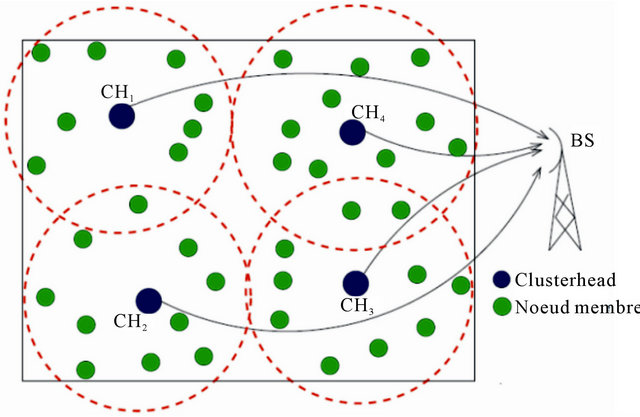
Figure 1. Considered network architecture [18].
The whole clusterheads (CH) constitute the second level; they merge the attentive messages transmitted by their members and send the created signal towards the base station. CH and its members form a cluster. A cluster is defined as being the coverage area of its CH.
The members as well as CHs have the same features (a limited battery in energy and two radios receiving/ transmitters: to communicate with the network of the first level and another for the communication with the base station). The base station forms the third level, it treats the received data.
The members of cluster communicate directly with their CHs (connectivity intra-cluster to 1 hop). CHs communicate directly with the base station. This communication procedure is defined in LEACH clustering algorithm [22] whose goal is to lower the energy consumption during the communication.
We suppose that the nodes of the first level work on the frequency channels 802.15.4 (zigbee). Indeed, four frequency channels are enough to sweep all the communication surface while being based on the principle of frequency re-uses. We also suppose that CHs use the protocol pile of standard 802.11 for their communication with the base station.
5. Model and Notation
We will model the RCSF by a graph  where V represents the whole of sensors and

represents the whole of wireless connections between nodes. R is the communication range, and D(U,v) defines the Euclidean distance between the nodes U and V.
The properties are the following:
• N: the number of nodes.
• ID (U): the identifier of node U.
• D (U): the connectivity degree of U.
• M (U): the mobility of U.
• Ec/com(U): power consumption by communication unit of U.
• Dis(U): the distance between the node U and the base station.
• Neigh (U): is the whole of nodes in the neighborhood of 1-hop of U.
• D (U): the degree U.
• Weight (U): the weight of U.
• State (U): state of U. We distinguish two states: “CH” (clusterhead) and “Nm” (nodes member)
• T: is the period of standby mode (deactivation period).
6. MED-BS Clustering Algorithm
In this section, we propose a new clustering algorithm called MED-BS (Mobility Energy Degree Distances to Base Station) Clustering Algorithm for the sensors networks of which the goal is the minimization of the power consumption in the cluster creation phase.
6.1. Mobility Model
Mobility is the leading cause of topology changes in the sensors networks. It should be essential to integrate mobility metric for the clusterheads election and the clusters’ formation.
We will define three mobility levels for sensors:
• Level 1: nodes speed is very weak in this case, speed lies between 0 and 5 km/h.
• Level 2: nodes speed is average, in this case, speed lies between 5 km/h and 20 km/h.
• Level 3: nodes speed is high, in this case, speed lies between 20 km/h and 44 km/h.
We suppose that the sensors speed is constant. The sensor mobility is characterized by the mobility level and can have the following values:
• M(U) = 1, if the node speed U belongs to first level.
• M(U) = 2, if the node speed U belongs to second level.
• M(U) = 3, if the node speed U belongs to third level.
We also suppose that sensors nodes know in advance their mobility levels and that the nodes having mean and high mobility will not take part in the clusterheads election phase. The purpose of this assumption is to maintain the stability of the structure. The consumed power by the mobility of nodes is not considered into account.
6.2. Energy Consumption Model
The energy consumption rate in the sensors networks represents the most important metric in the perform ances’ evaluation phase. This parameter depends on the used nodes’ characteristics (standby mode, nature of data processing, transmitted power, ···), and nodes behavior during the communication (retransmission, congestion, diffusion of the messages, ···) [32].
The consumed power by sensor is that the consumed power by these capture units, treatment units and communication units. So the energy consumption formula is defined as follows [25]:
 (1)
(1)
where:
• Ec/capture: is the energy consumed by a sensor during the capture unit activation. This energy depends primarily on the type of detected event (image, its, temperature···) and of the tasks to be realized by this unit (sampling, conversion ···).
• Ec/treatment: is the energy consumed by the sensor during the activation of its treatment unit.
• Ec/communication is the energy consumed by the sensor during the activation of its communication unit.
The consumed energy by sensors during communication is larger than those consumed by the treatment unit and the capture unit. Indeed, the transmission of a bit of information can consume as much as the execution of a few thousands instructions [33]. For that, we can neglect the energy of the capture unit, and the treatment unit compared to the energy consumed by the communication unit. In this case, the Equation (1) will be thus:
 (2)
(2)
The communication energy breaks up into emission energy and reception energy:
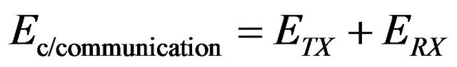 (3)
(3)
Referring to [34], the transmission energy and reception energy are defined as follows:
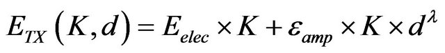 (4)
(4)
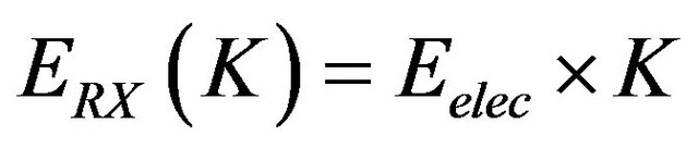 (5)
(5)
where:
• K: message length (bits).
• D: distance between transmitting node and receiving node (m).
• λ: of way loss exhibitor, .
.
• Eelec: emission /reception energy, .
.
• εamp: transmission amplification coefficient,  .
.
In [22], the authors compared the consumed power by a clusterhead by carrying out the aggregation of received messages with that consumed without aggregation. They showed that when the energy considered for aggregation is lower than a limits value (1 µJ/bit/signal), then, the transmission with aggregation requires a weaker energy than that without aggregation.
We suppose that the aggregation energy cost respects the limiting value introduced into [22]. The power consumed by a clusterhead during the transmission towards the base station will be thus:
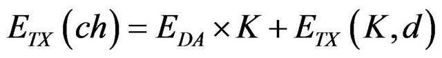 (6)
(6)
where EDA: power consumed during aggregation.
6.3. ClusterHeads Election Procedure
Step 1: Each node sends a message “hello” for the discovery of 1-hop neighborhood.
Step 2: Nodes having a low level of mobility (M(U) = 1) calculate their weights, the weight is calculated as follows:
 (6)
(6)
Two nodes do not having the same weight because of the distance parameter (Dis(U)).
Step 3: The nodes diffuse their weights towards their neighbors.
Step 4: The node which has the weakest weight is declared like clusterhead by putting its state = “CH” and sends a message “clusterhead_elected” (containing its identity) to its neighbors.
Step 5: The neighbors receiving this message, declare themselves like “Nm”, send to the clusterhead a message “clusterhead_accepted”, and record the identity of their clusterheads in their databases.
6.4. Particular Conditions
Condition 1: A node receiving two messages “clusterhead_elected” on behalf of both clusterheads, chooses that having the weakest weight.
Condition 2: A node having a worthless degree (not having neighbors), sends its data directly towards the base station and starts the “to join a new cluster” procedure (this procedure will be thereafter detailed).
Condition 3: An outgoing node (from the cluster), sends its data directly towards the base station and starts the “to join a new cluster” procedure.
Condition 4: A clusterhead checks its reserve of energy periodically, if the remaining energy is about 40% * initial energy, then the clusterhead starts the procedure of “change clusterhead” then is declared like “Nm”.
6.5. To Join New Cluster Procedure
Periodically, the base station sends to the disconnected nodes the list of clusterheads and their place. Each node calculates at each period its distances from different clusterheads, if a distance is ≤R, then it sends a message “hello” towards the concerned clusterhead. The clusterhead sends its ID and the node joins this cluster by sending a message “clusterhead_accepted”.
6.6. ClusterHeads Change Procedure
Step 1: The clusterhead sends to its neighbors a message “clusterhead-changes”, and is declared like “Nm”.
Step 2: The nodes having a low mobility calculate and send their weights Step 3: The node having the weakest weight is declared like “CH”, and diffuses a message “clusterhead_elected ”.
Step 4: The neighbors send to the clusterhead a message “clusterhead_accepted”, and record the identity of their clusterhead in their databases.
6.7. Sending Information towards the Base Station
Each member has one period of deactivation T. It awakes each time, collects information and sends it towards its clusterhead. The clusterhead aggregates received informations and sending the built message towards the base station.
7. Simulations Results
The results of our algorithm are getting using Matlab 7.0.1 in a computer Intel® Pentium® Dual CPU 1.86 Ghz with 1.99 Go of RAM.
The network of first level is composed of set of sensors. The number node in the sensor network varies between 10 and 200 nodes. The mobility of each sensor is supposed constant, and a speed is dedicated for each level of mobility: level 1:1 km/h, level 2:5 km/h and level 3:20 km/h. The initial energy for each sensor is equal to 0.5 J.
The simulation of our algorithm was carried out during 10 deactivation intervals T (standby mode) in a space of 150 m × 150 m and the range of the nodes (Tx-Arranges) varies between 20 m and 100 m. The size of a measured data package for sensors and envoy towards their clusterheads is 4000 bits.
During simulation, several metric were taken into account: the energy consumption, median number of clusterheads, median number of emitted packages towards the base station, average number of emitted packages towards the clusterheads, control traffic emitted/received during the clusters construction phase and the control traffic emitted/received during the data emission phase.
In this section, we will represent the results of our algorithm by varying the nodes range then we will compare our algorithm with LEACH algorithm while varying the size of the network each time.
7.1. Performances Evaluation: MED-BS Algorithm
In follows, we consider 100 nodes spaced in a geographical zone of 150 m × 150 m, the range of the nodes varies between 20 m and 100 m.
The following figure (Figure 2) represents the impact of energy consumption on tx-ranges. We can see that the energy consumption increases with the nodes’ transmission range. We also notice that this energy increases proportionally but slightly with the value of the tx-range; this is explained by the increase in the node tx-range which leads to an increase in the emission power and thus to the increase in the consumed power.
On the same figure, we can see that the percentage of the consumed power remains weak (about 0.088%) and does not exceed the 0.146% in the worst cases (100 m), these values remain reasonable for a network having 100 nodes.
Figure 3 represents the impact of clusterheads number on tx-ranges. We can notice that the clusterheads number falls regularly according to nodes’ tx-range. This is explained by the increase of tx-range which leads to the increase among neighbors (degree) for each node. Under these conditions, the number of members of clusterhead increases and by results, the number of created clusterheads too.
The following figure (Figure 4) shows the impact on the evolution of the median number of packages emitted towards the base station (resp. towards the cluster-
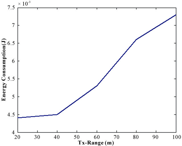
Figure 2. Energy consumption vs tx-range.
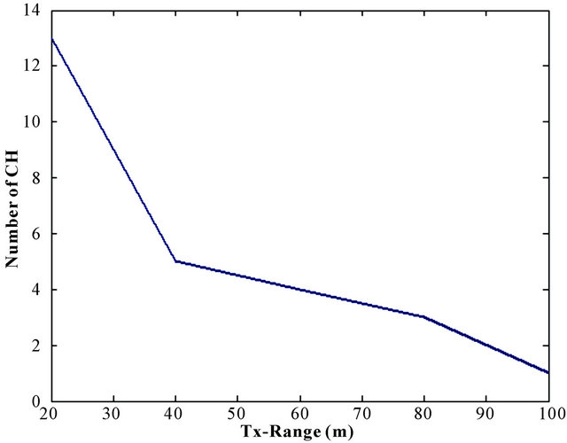
Figure 3. Number of clusterheads vs tx-range.
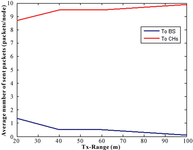
Figure 4. Average number of sent packets vs tx-range: 1. To base station and 2. To clusterheads.
heads) on tx-range. The number of packages sent towards the clus-terheads increases regularly with tx-ranges, that is due to the amplification of the clusterheads members by multi-plying their coverage areas.
The same figure shows that the shape of the second curve is opposed to that of the first. Indeed, the increase in the tx-range minimizes the number of the clusterheads created (Figure 3) and thereafter reduces the number of the sent packages towards the base station.
Figure 5 describes the evolution of the sent control traffic according to tx-ranges during clusters’ construction phase like after their construction. During the clusters’ construction phase, the control traffic is rather high, that is due to the messages “hello” transmitted at the time of the neighborhood discovery as well as the sent messages between each clusterhead and its members (“clusterhead-elected” and “clusterhead-accepted”). We can notice that the control traffic evolves with the increase in tx-ranges, and this is explained by the increase of neighbors’ number each time.
The same figure shows us after the clusters construction phase, the control traffic decreases according to the tx-range, the measured values are rather lower than those measured with the first phase. This pace shows well the stability of built structure throughout the data sending phase.
The same pace characterizes the received control traffic (Figure 6). The value of the received messages at the clusters construction phase is raised and arrives at 170 messages/node with a tx-range of 100 m, explained by the increase of neighbors’ number leads to the increase among messages “hello” received during the discovered neighborhood phase.
7.2. MED-BS vs Leach
Among the most known clustering algorithm in literature: we distinguish, LEACH algorithm. LEACH is a famous

Figure 5. Control traffic sent vs tx-range: 1. Before clusters construction and 2. After clusters construction.

Figure 6. Control traffic received vs tx-range: 1. Before clusters construction and 2. After clusters construction.
algorithm which goal is the minimization of the energy consumption in the sensors networks.
We wish in this part to compare MED-BS Clustering Algorithm with the LEACH clustering algorithm. The same energy and mobility models were considered for the two algorithms. LEACH was carried out during 10 successive towers, in parallel; MED-BS was carried out during 10 successive deactivation periods. The networks’ size tested varied between 10 and 200 nodes.
Figure 7 represents the impact of the median number of built clusterheads on the network cardinality. We notice that the number of clusterheads increases regularly with the network size.
The same figure shows that MED-BS Clustering Algorithm produces less clusterheads in most shared of cases (size between 40 and 200). For LEACH more clusterheads are necessary for a larger cardinality. For MED-BS, the same number of clusterheads can be used to manage a higher network size. That explains the effecttiveness of the structure created by MED-BS if a set of sensors is added.
Figure 8 represents the impact of average spent en-

Figure 7. Average number of clusterheads vs number of nodes: 1. MED-BS clustering algorithm and 2. Leach algorithm.
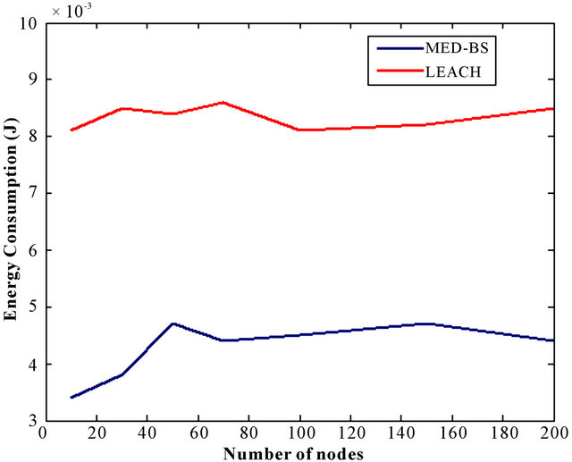
Figure 8. Energy consumption vs number of nodes: 1. MED-BS clustering algorithm and 2. Leach algorithm.
ergy by node on the network size. We can note that the values obtained by MED-BS are rather low compared to those obtained by LEACH. These results show that MED-BS is more effective and can prolong the network lifetime and ensure its good performance.
8. Conclusions
We presented in this paper a new clustering algorithm for the small-scale sensors networks called MED-BS. The main aim of our algorithm is the prolongation of the network lifetime; four parameters were taken into account for the choice of clusterheads: the nodes’ mobility, their power consumption, their degree and their distance from the base station.
The simulation results show that our algorithm is more effective in energy and build a stable structure being able to support new sensors without returning to the clusters rebuilding phase.
REFERENCES
- R. Kacimi, “Techniques de Conservation D’Energie Pour les Réseaux de Capteurs Sans Fil,” Ph.D., Toulouse University, Toulouse, 2009.
- H. Cuong, “Optimisation D’Accès au Médium et Stockage de donnEes Distribuées Dans les Réseaux de Capteurs,” Ph.D., University of Franche-Comté, Besançon, 2008.
- A. Makhoul, “Réseaux de Capteurs: Localisation, Couverture et Fusion de Données,” Ph.D., university of FrancheComté, Besançon, 2008.
- L. Samper, “Modélisations et Analyses de Réseaux de Capteurs,” Ph.D., Verimag Laboratory, Grenoble, 2008.
- Y. Yaser, “Routage pour la Gestion de l’Energie ans les Réseaux de Capteurs Sans Fil,” Ph.D., University of Hight Alsase, Mulhouse, 2010.
- P. Parrend, “Localisation dans les Réseaux de Capteurs,” Ph.D., Californie University, Berkeley, 2005.
- K. Beydoun, “Conception d’un Protocole de Routage Hiérarchique Pour les Réseaux de Capteurs,” Ph.D., University of Franche-Comté, Besançon, 2009.
- K. Drira, H. Kheddouci and N. Tabbane, “Topologie Dynamique Virtuelle pour le Routage dans les Réseaux Mobiles Ad Hoc,” SETIT 2007, Tunisia, 2007, pp. 25-29.
- M. Ayaz, I. Baig, A. Abdullah and I. Faye, “A Survey on Routing Techniques in Underwater Wireless Sensor Networks,” Journal of Network and Computer Applications, Vol. 34, No. 6, 2011, pp. 1908-1927. doi:10.1016/j.jnca.2011.06.009
- M. Yarvis, N. Kushalnagar, H. Singh, A. R. Garajan, Y. Liu and S. Singh, “Exploiting Heterogeneity in Sensor Networks,” Proceedings of IEEE 24th Annual Joint Conference of the IEEE Computer and Communications Societies, Vol. 2, 2005, pp. 878-890. doi:10.1109/INFCOM.2005.1498318
- Z. Hongwei and A. Arora, “Gs3: Scalable Self-Configuration and Self-Healing in Wireless Networks,” Proceedings of the 21 Annual Symposium on Principles of Distributed Computing, Mobile and Wireless Communications Network, USA, 2002.
- G. Gupta and M. Younis, “Load-Balanced Clustering of Wireless Sensor Networks,” Proceedings of the IEEE International Conference, Vol. 3, 2003, pp. 1848-1852.
- C. P. Low, C. Ping, C. Fang, J. Mee and Y. H. Ang, “Load-Balanced Clustering Algorithms for Wireless Sensor Networks,” IEEE International Conference on Communications, Glasgow, 24-28 June 2007, pp. 3458-3490.
- T. Neeta, G. Elangovan, S. Iyengar and N. Balakrishnan, “A Message-Efficient, Distributed Clustering Algorithm for Wireless Sensor and Actor Networks,” IEEE International Conference on Multisensor Fusion and Integration for Intelligent Systems, Heidelberg, September 2006, pp. 53-58.
- L. Qing, Q. Zhu and M. Wang, “Design of a Distributed Energy-Efficient Clustering Algorithm for Heterogenous Wireless Sensor Networks,” Computer Communications, Vol. 29, No. 12, 2006, pp. 2230-2237. doi:10.1016/j.comcom.2006.02.017
- W. N. Richard and A. Boukerche, “Mobile Data Collector Strategy for Delay—Sensitive Applications over Wireless Sensor Networks,” Computer Communications, Vol. 31, No. 5, 2008, pp. 1028-1039. doi:10.1016/j.comcom.2007.12.024
- D. Kumar, D. Trilok, C. Aseri and R. B. Patel, “EEHC: Energy Efficient Heterogeneous Clustered Scheme for Wireless Sensor Networks,” Computer Communication, Vol.32, No. 4, 2009, pp. 662-667. doi:10.1016/j.comcom.2008.11.025
- C. T. Kone, “Conception de l’Architecture d’un Réseau de Capteurs sans Fil de Grande Dimension,” Ph.D., University of Henri Poincaré, Nancy, 2011.
- A. Ephremides, J. E. Wieselthier and D. J. Baker, “A Design Concept for Reliable Mobile Radio Networks with Frequency Hopping Signaling,” Proceedings of the IEEE, Vol. 75, No. 1, 1987, pp. 56-73. doi:10.1109/PROC.1987.13705
- G. Mario and J. T.-C. Tsai, “Multicluster, Mobile, Multimedia Radio Network,” Wireless Networks, Vol. 1 No. 3, 1995, pp. 255-265 doi:10.1007/BF01200845
- A. D. Amis, R. Prakash, T. H. P. Vuong and D. T. Huynh, “Max-Min d-Cluster Formation in Wireless Ad Hoc Networks,” Proceedings of 19th Annual Joint Conference of the IEEE Computer and Communications Societies, Vol. 1, 2000, pp. 32-41.
- W. R. Heinzelman, A. Chandrakasan and H. Balakrishnan, “Energy-Efficient Communication Protocol for Wireless Microsensor Networks,” Proceedings of IEEE 33rd Hawaii International Conference on System Sciences, USA, 4-7 January 2000. doi:10.1109/HICSS.2000.926982
- W. B. Heinzelman, “Application-Specific Protocol Architectures for Wireless Networks,” Ph.D, B. S. Cornell University, New York, 2000.
- C. Mainak, K. Das and D. Turgut, “Wca: A weighted Clustering Algorithm for Mobile Ad Hoc Networks,” Cluster Computing, Vol. 5, No. 2, 2002, pp. 193-204. doi:10.1023/A:1013941929408
- N. Mitton, A. Busson and E. Fleury, “Self-Organization in Large Scale Adhoc Networks,” Mediterranean Ad Hoc Networking Workshop (Med-Hoc-Net’04), Bodrum, 2004.
- Y. Ossama and S. Fahmy, “HEED: A Hybrid EnergyEfficient Distributed Clustering Approach for Ad Hoc Sensor Networks,” IEEE Transactions on Mobile Computing, Vol. 3, No. 4, 2004, pp. 366-379. doi:10.1109/TMC.2004.41
- C. M. Duan and F. Hong, “A Distributed Energy Balance Clustering Protocol for Heterogeneous Wireless Sensor Neworks,” International Conference on Wireless Communications, Networking and Mobile Computing, Shanghai, 21-25 September 2007, pp. 2469-2473.
- Z. H. Yu, Y. Liu and Y. L. Cai, “Design of an Energy- Efficient Distributed Multi-Level Clustering Algorithm for Wireless Sensor Networks,” Proceedings of IEEE 4th International Conference: Wireless Communications, Networking and Mobile Computing (WiCOM’08), Dalian, 12-14 October 2008, pp. 1-4.
- L. Mohamed, “Diffusion et Couverture Basées sur le Clustering Dans les Réseaux de Capteurs: Application à la Domotique,” Ph.D., University of Franche-Comté, Besançon, 2009.
- G. Chalhoub, “Les Réseaux de Capteurs Sans Fil”, Ph.D, University of Clermont, Auvergne, 2010.
- M. Khan and J. Misic, “On the Lifetime of Wireless Sensor Networks,” ACM Transactions on Sensor Networks (TOSN), Vol. 5, No. 5, 2009, Article ID: 5.
- V. Raghunathan, C. Schurgers, S. Park and M. B. Srivastava, “Energy-Aware Wireless Micro-Sensor Networks,” IEEE Signal Processing Magazine, Vol. 19 No. 2, 2002, pp. 40-50. doi:10.1109/79.985679
- G. J. Pottie and W. J. Kaiser, “Wireless Integrated Network Sensors,” Communications of the ACM, Vol. 43, No. 5, 2000, pp. 51-58. doi:10.1145/332833.332838
- M. J. Handy, M. Haase and D. Timmermann, “Low Energy Adaptive Clustering Hierarchy with Deterministic Cluster-Head Selection,” Proceedings of the IEEE 4th International Workshop Mobile and Wireless Communication Network, Germany, 2002, pp. 368-372. doi:10.1109/MWCN.2002.1045790