Wireless Sensor Network
Vol.5 No.1(2013), Article ID:27484,7 pages DOI:10.4236/wsn.2013.51001
An Energy Efficient Color Based Topology Control Algorithm for Wireless Sensor Networks
Institute of Engineering and Computing Sciences, University of Science and Technology Bannu, Bannu, Pakistan
Email: asghar_surani@yahoo.com
Received November 2, 2012; revised December 9, 2012; accepted December 24, 2012
Keywords: Sensor; Topology Control; Energy Efficiency; Energy Conservation
ABSTRACT
Wireless Sensor Networks (WSNs) are universally being used and deployed to monitor the surrounding physical environments and detail events of interest. In wireless Sensor Networks energy is one of the primary issues and requires energy conservation of the sensor nodes, so that network lifetime can be maximized. To minimize the energy loss in dense WSNs a Color Based Topology Control (CBTC) algorithm is introduced and implemented in Visual Studio 6.0. The results are compared with Traditional dense WSNs. In the evaluation process it was observed that the numbers of CPU ticks required in traditional WSNs are much more than that’s of CBTC Algorithm, both in Normal and Random deployments. So by using CBTC, delay in network can be minimized. Using CBTC algorithm, the energy conservation and removal of coverage holes was also achieved in the present study.
1. Introduction
Now-a-Days there is an increased interest in the use of wireless sensor networks (WSNs) in different fields of life. They are used for different applications such as forest monitoring, disaster management, space exploration, factory automation, secure installation, border protection, and battlefield surveillance [1,2]. Wireless sensor network is a network of large collection sensor nodes that work together in cooperative manner. A sensor network is a computer network consisting of a large number of sensor nodes [3]. Usually these devices are small and inexpensive, so that they can be produced and deployed in large numbers [1] as shown in Figure 1.
Almost every sensor node consists of the following components [4].
1) Memory;
2) Controller;
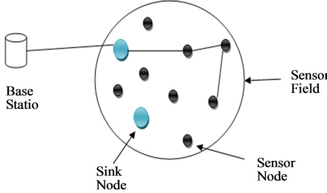
Figure 1. Typical Wireless Sensor Network.
3) Power supply;
4) Communication device;
5) Sensing device.
According to Jason Lester Hill [5], the whole concept of WSNs is based on a simple mathematical equation:
Sensing + Computation + Radio Operation = Thousands of potential applications.
In a sensor node, these three activities are the main sources of energy consumption. But in all these three sources, energy loss due to radio operation is the maximum one [6].
According to Prithwish Basu [7], WSNs can be classified into the following two categories:
§ Query-driven;
§ Event-driven.
In the query-driven WSNs, a user submits a query from a Base Station node. The query is broadcasted through the network and sensors that are related to the query or satisfy the query and response to the Base Station.
In event-driven WSNs, each sensor sends data to Base Station or Data Collection Center or Sink nodes whenever it detects a certain event.
The sensor can be found in four different states i.e. sensing, relaying, sleeping and dead [8], as described below.
Sensing: When a node is in a sensing mode then it monitors the source using an integrated sensor. It stores the required information in a small buffer memory and then sends it to the Base Station.
Relaying: In relaying state, a node receives data from other nodes and forwards it towards their destination.
Sleeping: In this case, most of the sensor nodes are either shutdown or work in low-power mode. A sleeping node does not participate in either sensing or relaying. However, it “wakes up” from time to time and listens to the communication channel in order to answer requests from other nodes. Upon receiving a request, a state transition to “sensing” or “relaying” may occur.
Dead: It is that state of node in which it is no longer available to the sensor network. It has either used up its energy or has suffered vital damage. From dead state it cannot be revived to any other state.
2. Related Work and Background
The most important part of sensor network is deployment and connectivity of nodes where they work alone in unattended environments. In most cases the WSNs contains hundreds of nodes that operate on small built-in batteries. Low power capacities of sensor node results in limited coverage and communication range for sensor nodes as compare to other mobile devices [9]. A sensor node stops working when it runs out of energy and thus a WSN may be structurally damaged if many sensors exhaust their onboard energy supply [10]. Because of the limited energy storage capability of sensor nodes, Energy consumption is one of the most challenging aspects of these networks and different strategies and protocols deals with this area. In power limited wireless network research, the main goal is to achieve minimum communication energy consumption [11].
WSNs consist of many nodes which are deployed closely to each other. A single node has many neighboring nodes and every node can directly communicate with their neighbor nodes. Due to this, nodes will consume lot of energy. Closely deployed nodes can create many problems like [4]§ Energy loss;
§ Load on a MAC protocol;
§ Volatility in Routing Protocol.
According to Cardei, M. and Wu, J [12], the coverage of wireless sensor node can be estranged into three classes; area coverage (how to cover an area with the sensors), point coverage(coverage for a set of points of interest) and barrier coverage (decreasing the probability of undetected saturation is the main issue in barrier coverage).
Most of the coverage problems in WSNs are due to the following three main reasons; not enough sensors to cover the whole region of interest, limited sensing range and random deployment [13].
Many techniques can be used to restrict the nodes that are considered as neighbors. This can be done by controlling transmission power, by introducing hierarchies in the network and signaling out some nodes to take over certain coordination tasks or by simply turning off some nodes for a certain time. Therefore, by use of topology control techniques, the topology of the network is deliberately restricted in order to decrease the power consumption [4]. Many different techniques can be classified as topology control mechanisms. One of the simplest types of topology control issues deals with finding the minimum value for transmitting range such that a certain network wide property is satisfied [14].
According to [15,16] the problems in sensor node deployment are categorized in the following four classes; 1) Node Problems that involve only a single node; 2) Link Problems that involve two neighboring nodes and the wireless link between them; 3) path problems that involve three or more nodes and a multi-hop path formed by them; and 4) global problems that are properties of the network as a whole.
Different topology control techniques are studied for wireless sensor networks and have come in observation that some scholars minimized link interference when network topology is modeled, someone uses Euclidean minimum spanning tree, other Sleep-based Topology Control [17,18]. In [19] it is discussed that when network topology is modeled as a connectivity graph in which each wireless link is either connected or disconnected, but the energy efficient topology control is that one which has less connected sets. Zhang and Hou proposed a method for maintaining sensor coverage and communication connectivity by utilizing a WSN with a minimal number of Sensor Nodes [20].
3. Problem Statement and Objectives
Sensor node deployment and topology control (TC) are the two most important factors that can affect the performance of WSNs if not handled properly. Worse deployment and TC of wireless sensor nodes creates many problems like loss of energy, coverage hole and delay in network.
In this paper, Color Based Topology Control (CBTC) algorithm is designed for wireless sensor networks in order to achieve maximum lifetime of sensor nodes, minimize delay in the network and to remove coverage holes in network.
4. Color Based Topology Control Algorithm
In topology control, there are multiple taxonomy of approaches to topology control discussed by [21] given in Figure 2.
In densely deployed and fully connected WSNs as shown in Figure 3, large amount of energy is consumed due to multiples neighbor’s node.
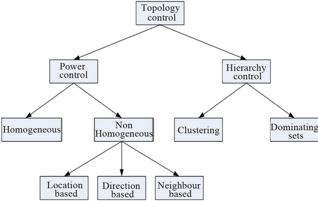
Figure 2. Multiple taxonomy of approaches to topology.
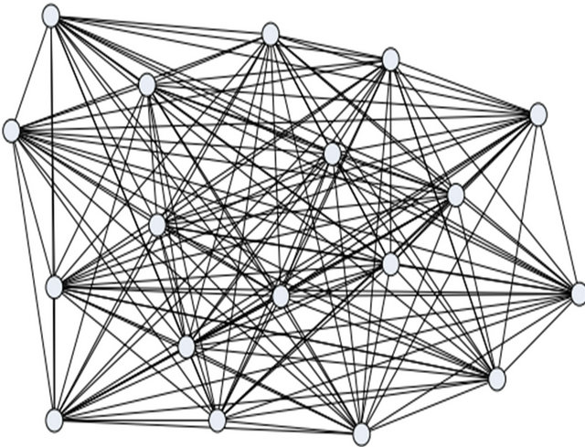
Figure 3. Fully connected WSN.
To control multiple neighbors’ nodes different strategies are used. In some approaches neighbors are controlled but energy consumption and coverage holes are created or after some time energy holes are produced. In some cases, it was observed that if coverage holes are removed then the topology cannot be controlled properly. In this paper, a topology control was designed in which energy consumption due to multiple neighbors’ nodes was minimized and coverage holes were removed.
4.1. New Topology Control for WSNs
For reducing the numbers of neighbor nodes and the numbers of links between sensor nodes, a new topology control algorithm is introduced, known as “Color Based Topology Control (CBTC) algorithm”. Through this algorithm, an identifier i.e. “color_flag” is used inside the code area of the sensor node, denoting the color of that node. Five color_flags are used i.e. blue, black, red, green, and white. All the sensors nodes are sensitive for some particular application, i.e. humidity, temperature or pressure etc. A node of same color flag can sense another node in its coverage area and communication between them is possible. The topology control is supposed to be used in two scenarios i.e. Uniform Deployment and Random Deployment of nodes. In case of Random Deployment it can select node of other color.
Suppose that the sensors nodes are deployed in uniformed way; such that every node of the same color_ flag is equidistance from each other and there is no coverage problem. Communication between same color nodes is possible. Suppose that if someone wants to deploy 5000 nodes, then there must be 1000 nodes of each color_flag. This scenario is shown in Figure 4.
In the above and all other figures of CBTC, we denote Black node by 1, Green by 2, White by 3, Blue by 4 and Red by 5.
When network size is large or the sensor field is remote and hostile, random sensor deployment might be the only choice e.g. scattered from an aircraft. Suppose that sensor nodes are deployed in random manner then there may be the possibility that the distance between two nodes of same color_flag is greater than their required range (far from the coverage area of some other sink or sensor node). But there exist a node of other color flag. In such scenario, a node of other color flag can be selected within its coverage area. This scenario is shown in Figure 5.
4.2. Removal of Coverage Hole
In sensor network when a node; which is on the way to some sink node become dead then there occur a coverage hole. Through this coverage hole other nodes cannot transmit their data to the sink node as shown in Figure 6. The encircle node represent dead node due to which coverage hole is created.
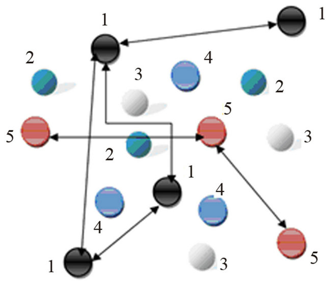
Figure 4. Uniform deployment of nodes
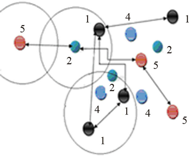
Figure 5. Random deployment of nodes.
To remove this problem in the color based topology algorithm, when a node of some color, suppose the node of color flag “blue” becomes dead, then it should work by choosing some node of other color flag within its coverage area. As shown in Figure 7.
4.3. Mathematical Approach of the CBTC
In dense deployed WSNs all node have the same capabilities. As a result, loss of energy problem occurs due to a lot of communication whenever an event occurs.
The algorithm can be explained with the help of the following mathematical functions.

where A= {blue, green, white, black, red}
________________________________Function No. 1 f(x) = y, if f(x) ≠ x and y is the shortest among B. where B = A – x
________________________________Function No. 2 Equation (1) shows that if the value of “x” is equal to the value in the f(x), i.e.
Sensing Node’s Color = Sink Node’s Color
Moreover the color of the sensing node as well as other sink nodes are within the set A= {blue, green, white, black, red} then it will start communication with its color nodes.
In case, if f(x) it will follow the Equation (2) in which it will re-sense a node of other color for communication, other color node will be within the set B {blue, green, white, black, red}—its own color. The re-sensed node should be the shortest of all other colors node.
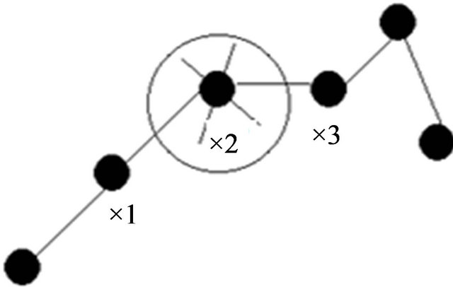
Figure 6. Coverage hole.
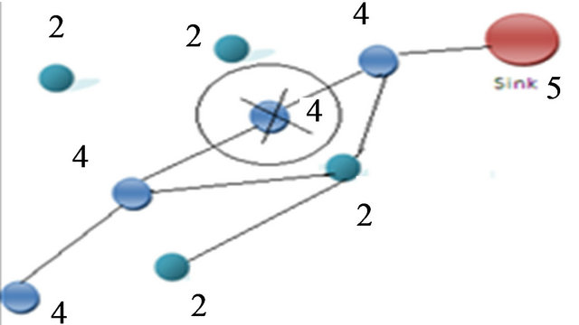
Figure 7. Removal of coverage hole.
4.4. Pseudocode for CBTC
Case No. 1
START CF: = COLOR CFX: = GetColor (X)
IF CF = CFX THEN TRANSMISSION () ↔ X END IF END
Case No. 2
START CF: = COLOR CFX: = GetColor (X)
IF CF = CFX THEN TRANSMISSION () ↔ X ELSE RESENSE (COLOR)
S = SHORTESTNODE ()
TRANSMISSION () ↔ S END IF END Note:
CF means color_flag CFX means color_flagof X
4.5. Flow Chart of CBTC
The execution flow of the CBTC algorithm is shown in a flowchart given in Figure 8.
In the flowchart CFC means color flag of current node and CFX means color flag of node “X”.
5. Evaluation of CBTC
Besides formal analysis of the CBTC algorithm, we employed implementation and evaluation of the CBTC algorithm in Visual Studio 6.0 to compare the performance between traditional WSNs and Color Based WSNs. We focused on the energy-conservation and delay in networks. The evaluation was done in Visual Studio 6.0 installed over Intel®, Pentium® 4, CPU 3.00 GHz, 2.99 GHz, with 512 MB of RAM running on 32 bits Operating System (Windows XP).
Evaluation of CBTC algorithm was done both in random and uniform distribution of nodes. In the evaluation 5000 nodes were considered (Because for less numbers of nodes the clock ticks generated by CPU are very short and accurate results could not be concluded). Node No. 2500 was considered as a base station. If an event occurs near to base station then the base station will receive the message quickly otherwise it will take time for propagation.
Every event was evaluated by all the three types of deployments i.e. T-WSN, CBTC-N and CBTC-R and results were compared.
5.1. Evaluation of CBTC w.r.t Time
For reducing delay in network in CBCT, time of propagation is measured and compared with T-WSN. Time is measured in clock-ticks generated by CPU.
A typical execution of the implemented program is given in Figures 9 and 10.
As from single experiment we cannot conclude result confirmedly so we performed and compared five experiments i.e. repeatedly execute the program five times, for five different nodes where the event has occurred, like
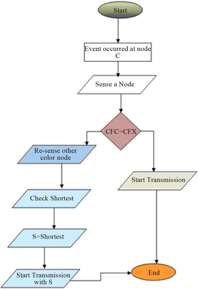
Figure 8. Flow chart of CBTC algorithm.
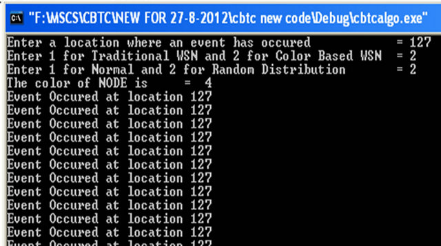
Figure 9. Typical execution screen of random deployment in CBCT (1).
shown in Figure 11. For each event we observed clockticks of CPU as given in Table 1.
The graph comparing the time ticks of different events is obtained from the above data, and shown in Figure 11.
In the above figure T-WSN stands for Traditional Wireless sensor Network, in CBTC-N and CBTC-R, N and R stands for Normal and Random deployments. It is clear from the Figure 11 that numbers of CPU ticks required to T-WSN is much larger than other two types of CBTC. In CBTC, the CBTC-R takes larger time as compared to CBTC-N due to re-sensing and selecting other color node, in case of none-availability of its own color node.
5.2. Evaluation of CBTC w.r.t Energy
Most of the researches shown that energy consumption
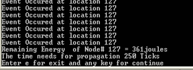
Figure 10. Typical execution screen of random deployment in CBCT (2).
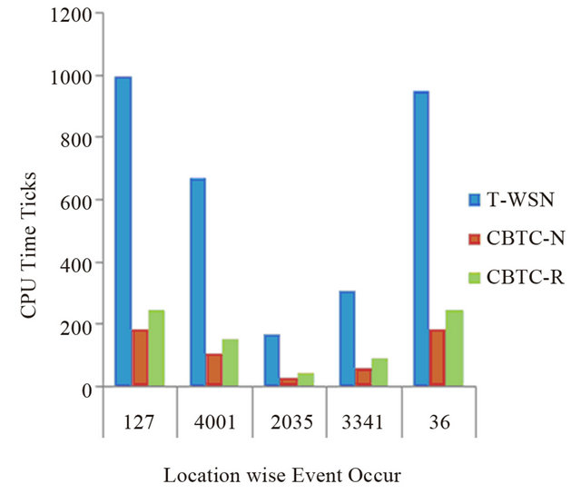
Figure 11. Comparison of T-WSN and CBTC with respect to time.
Table 1. Evaluation w.r.t time.

of sensor node is dominated by communication [22,23]. According to Gitanjali Shinde and Swati Joshi [24] the energy consumption is almost directly proportional to the time of communication between sensor nodes. If the time of communication is much then lots of energy will be consumed. In the evaluation 400 Joules energy was given to every sensor node then the consumption of energy with respect to different events with different locations are given in Table 2.
The graph comparing the remaining energy of different node, after the different events are occurred is obtained from the above data, and shown in Figure 12.
It is clear from the Figure 12 that energy consumed by T-WSN is much greater CBTC algorithm. In CBTC, the CBTC-R takes greater amount of energy as compared to CBTC-N because of re-sensing and selecting other color node due to none-availability of its own color node. From the above figure we concluded that energy consumption in CBTC algorithm is much less than traditional dense WSNs.
5.3. Evaluation of CBTC w.r.t No. of Packets
A sensor node play two roles in the WSNs one is sending its own sensed data and other is forwarding the data sensed of other sensors nodes. If each node has to send the same amount of data then the energy consumed by each node is identical [25]. Now we observed at the number of packet received in traditional Wireless Sensor Network, in CBTC-N and CBTC-R, these are shown in Table 3.
Table 2. Evaluation w.r.t energy.
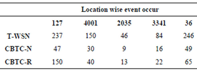
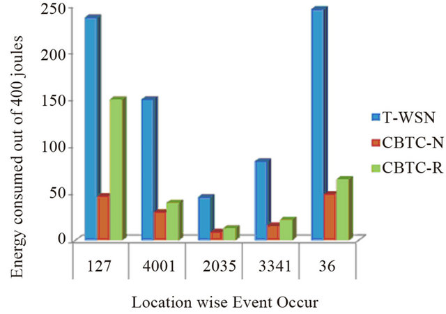
Figure 12. Remaining Energy after event occurred.
Table 3. Evaluation w.r.t number of packet received.
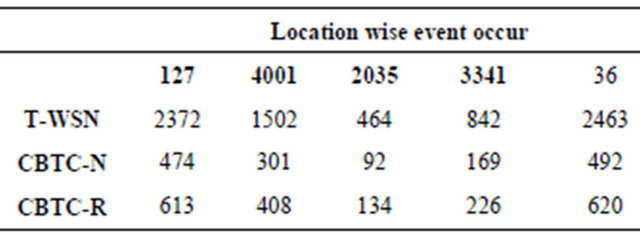
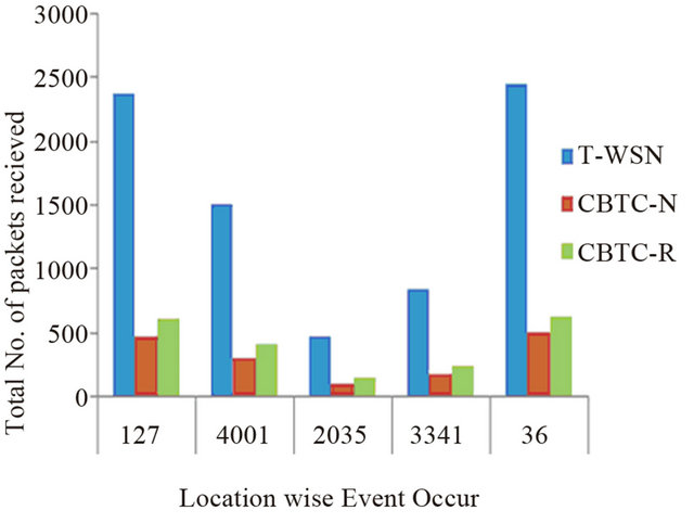
Figure 13. Comparison of T-WSN and CBTC with respect to numbers of packets received.
The graph comparing the numbers of packets received during different events are occurred is obtained from the above data, and shown in Figure 13.
From the above figure we concluded that the numbers of packets received in traditional dense WSNs are much more than CBTC-R and CBTC-N. And if fewer packets received and transmitted then less amount of energy will be consumed.
6. Conclusions
In the evaluation process it was observed that the numbers of CPU ticks required to T-WSNs are much more than that of CBTC-N and CBTC-R. So by using CBTC algorithm, delay the in network can be reduced and the network will be more efficient. Moreover in the evaluation it was also determined that the energy consumption in T-WSN is much more than that of CBTC-N and CBTC-R. By using CBTC algorithm energy can be conserved. Total numbers of packets received in T-WSN are much more than that of CBTC algorithm. So in all aspects i.e. time, energy and no. of packets the CBTC is better than T-WSNs.
Moreover the problem of coverage hole is also resolved in CBTC by choosing node of other color within its coverage area, for sending its data.
REFERENCES
- I. F. Akyildiz, W. Su, Y. Sankarasubramaniam and E. Cayirci, “Wireless Sensor Networks: A Survey,” Computer Networks, Vol. 38, No. 4, 2002, pp. 393-422. doi:10.1016/S1389-1286(01)00302-4
- C.-Y. Chong and S. P. Kumar, “Sensor Networks: Evolution, Opportunities, and Challenges,” Proceedings of the IEEE, Vol. 91, No. 8, 2003, pp. 1247-1256. doi:10.1109/JPROC.2003.814918
- http://en.wikipedia.org/wiki/Sensor_Networks
- H. Karl and A. Willig, “Protocols and Architectures for Wireless Sensor Networks,” John Wiley & Sons, Hoboken, 2005. doi:10.1002/0470095121
- J. L. Hill, “System Architecture for Wireless Sensor Networks,” University of California, Berkeley, 2003.
- I. Demirkol, C. Ersoy and F. Alagoz, “MAC Protocols for Wireless Sensor Networks: A Survey,” IEEE Communication Magazine, Vol. 44, No. 4, 2006, pp.115-121. doi:10.1109/MCOM.2006.1632658
- P, Basu and J. Redi, “Effect of Overhearing Transmissions on Energy Efficiency in Dense Sensor Networks,” Proceedings of the 3rd International Symposium on Information Processing in Sensor Networks, Berkeley, 26-27 April 2004, pp. 196-204.
- W. Li and C. G. Cassandras, “A Minimum-Power Wireless Sensor Network Self-Deployment Scheme,” IEEE Wireless Communications and Networking Conference, Vol. 3, 2005, pp. 1897-1902.
- A. Roy and N. Sarma, “Energy Saving in MAC Layer of Wireless Sensor Networks: A Survey,” National Workshop in Design and Analysis of Algorithm (NWDAA), Tezpur University, Assam, 2010, pp. 961-994.
- M. Younis and K. Akkaya, “Strategies and Techniques for Node Placement in Wireless Sensor Networks: A Survey,” Ad Hoc Networks, Vol. 6, No. 4, 2008, pp. 621-655. doi:10.1016/j.adhoc.2007.05.003
- C. Suh, Y.-B. Ko, C.-H. Lee and H.-J. Kim “Numerical Analysis of the Idle Listening Problem in IEEE 802.15.4 Beacon-Enable Mode,” 1st International Conference on Communications and Networking in China, Beijing, 25-27 October 2006, pp. 1-5.
- M. Cardei and J. Wu, “Coverage in Wireless Sensor Networks,” In: M. Ilyas and I. Mahgoub, Handbook of Sensor Networks: Compact Wireless and Wired Sensing Systems, CRC Press, Leiden, 2005.
- N. A. Ab. Aziz, K. Ab. Aziz and W. Z. W. Ismail, “Coverage Strategies for Wireless Sensor Networks,” World Academy of Science, Engineering and Technology, Vol. 50, 2009, pp. 145-150.
- P. Santi, “Topology Control in Wireless Ad Hoc and Sensor Networks,” John Wiley & Sons, Hoboken, 2005, pp. 27-95. doi:10.1002/0470094559.ch3
- M. Ringwald, K. Romer and A. Vitaletti, “Passive Inspection of Wireless Sensor Networks,” Proceedings of the 3rd International Conference on Distributed Computing in Sensor Systems, Vol. 4549, 2007, pp. 205-222.
- J. Beutel, K. Romer, M. Ringwald and M. Woehrle, “Deployment Techniques for Sensor Networks,” Signals and Communication Technology, 2009, pp. 219-248. doi:10.1007/978-3-642-01341-6
- G. N. Purohit and U. Sharma, “Topology Control for Energy Conservation in Wireless Sensor Network,” International Journal of Contemporary Mathematical Sciences, Vol. 7, No. 5, 2012, pp. 227-239.
- Y. Y. Zhou and M. Medidi, “Sleep-Based Topology Control for Wakeup Scheduling in Wireless Sensor Networks,” 4th Annual IEEE Communications Society Conference on Sensor, Mesh and Ad Hoc Communications and Networks, San Diego, 18-21 June 2007, pp. 304-313.
- J. Ma, Q. Zhang, C. Qian and L. M. Ni, “Energy-Efficient Opportunistic Topology Control in Wireless Sensor Networks,” Proceedings of the 1st International MobiSys Workshop on Mobile Opportunistic Networking, San Juan, 11 June 2007, pp. 33-38.
- S. Tanabe, K. Sawai and T. Suzuki, “Sensor Node Deployment Strategy for Maintaining Wireless Sensor Network Communication Connectivity,” International Journal of Advanced Computer Sciences and Applications, Vol. 2, No. 12, 2011, pp. 140-146.
- P. Santi, “Topology Control in Wireless Ad Hoc and Sensor Netowrk,” ACM Computing Surveys, Vol. 37, No. 2, 2005, pp. 164-194. doi:10.1145/1089733.1089736
- J. M. Kahn, R. H. Katz and K. S. J. Pister, “Next Century Challenges: Mobile Networking for Smart Dust,” Proceedings of the 5th Annual ACM/IEEE International Conference on Mobile Computing and Networking, Seattle, 15-19 August 1999, pp. 263-270.
- Y. Yu, V. K Prasanna and B. Krishnamachari, “Energy minimization for Real-Time Data Gathering in Wireless Sensor Networks,” IEEE Transactions on Wireless Communications, Vol. 5, No. 11, 2006, pp. 3087-3096. doi:10.1109/TWC.2006.04709
- G. Shindeand and S. Joshi, “Wireless Sensor Network with DCDD,” 2012 International Conference on Information and Network Technology, Vol. 37, 2012, pp. 122- 126.
- J. Lian, K. Naik and G. B. Agnew, “Data Capacity Improvement of Wireless Sensor Networks Using Non-Uniform Sensor Distribution,” International Journal of Distributed Sensor Networks, Vol. 2, No. 2, 2006, pp. 121-145.