Wireless Sensor Network
Vol. 4 No. 11 (2012) , Article ID: 24692 , 7 pages DOI:10.4236/wsn.2012.411037
An Average Distance Based Self-Relocation and Self-Healing Algorithm for Mobile Sensor Networks
Department of Electrical and Computer Engineering, Florida International University, Miami, USA
Email: yqu002@fiu.edu, georgako@fiu.edu
Received September 28, 2012; revised October 25, 2012; accepted November 2, 2012
Keywords: Mobile Sensor Network; Coverage; Self-Relocation; Self-Healing
ABSTRACT
The sensing coverage of a wireless sensor network is an important measure of the quality of service. It is desirable to develop energy efficient methods for relocating mobile sensors in order to achieve optimum sensing coverage. This paper introduces an average distance based self-relocation and self-healing algorithm for randomly deployed mobile sensor networks. No geo-location or relative location information is needed by this algorithm thereby no hardware such as GPS is required. The tradeoff is that sensors need to move longer distance in order to achieve certain coverage. Simulations are conducted in order to evaluate the proposed relocation and self-healing algorithms. An average of 94% coverage is achieved in the cases that we are examined with or without obstacles.
1. Introduction
Nowadays sensors can be miniaturized due to the development of new technologies such as MEMS. Miniaturized sensors can be carried by small robots thereby becoming mobile. Mobile sensor networks have both military and civilian applications. Typical military applications are surveillance and reconnaissance. Similar civilian applications exist for homeland security and property protection exist [1,2]. The mobility of each node enables the self-deployment and self-healing of such sensor networks. Often sensors are randomly deployed in situations where people cannot deploy them precisely, due to environmental restrictions and other conditions. However, applications, such as, surveillance and reconnaissance, always require that sensors provide the best coverage. The key issue is how to deploy the sensors in an unknown environment so that we maximize their performance as well as utilize their energy efficiently.
The coverage optimization of sensor networks is an active topic. For non-mobile sensor networks Genetic Algorithms (GAs) have been used to find optimal locations for sensors that provide the best coverage and save energy in order to prolong the lifetime of the sensors [3-6]. GA methodologies work very well when the environment is known. However, they require a powerful central node that runs the optimization algorithm before sensors are deployed. Therefore, GAs cannot be used as distributed algorithms in the case of power limited sensors. Methods that achieve even distribution of the sensors have been developed for mobile sensor networks. For example, the potential field algorithm was introduced in [7]. Specifically, in [7] a sensor moves according to the potential field generated by the other sensors. Other even distribution methods include the virtual force method [8], the density control method [9] and the fluid model based method [10]. Also, a relocation algorithm that deals with coverage healing has been presented in [11]. This algorithm focuses on finding the redundant sensors and moves them in order to heal the uncovered area with the least traveled distance. All the relocation algorithms listed above need to know the sensors’ location or relative location each time they run. GPS is a popular way to find the geo-location of sensors. Geo-location information is very important in surveillance applications, but GPS systems consume a great amount of power. Large amount of power is also consumed when sensors transmit their location to other sensors during the steps of deployment algorithms that require the geo-location information. Also, the cost and accuracy of GPS need to be considered. For example, the GPS kits sold by TI that has accuracy around 3 meters cost $40 each [17].
One way to reduce a sensor’s energy consumption is to reduce its sensing range. This has been discussed for target coverage in non-mobile sensor networks [12]. According to our knowledge, no previous work has considered adjusting the sensing range to save energy in problems that involve the coverage optimization of mobile sensor networks. This paper introduces a self-deployment and self-healing algorithm for mobile sensors based on the average distance between sensors. Adjustable sensing range is also used in order to save energy and prolong the lifetime of sensor networks. No location information is needed by our algorithm thereby requiring no geo-location hardware. The remainder of this paper is organized as follows: 1) Section 2 describes our assumptions and the sensor relocation algorithm, 2) Section 3 presents our results and analysis, and 3) Section 4 summarizes the conclusions.
2. Assumptions and Algorithm Description
2.1. Assumptions
For our algorithm to work the following conditions must be satisfied:
• All sensors, which exist within a sensors’ communication range Rc, can measure the signal strength when they receive a signal from other sensors. Each sensor uses same transmission power and has same communication range.
• The sensing area of each sensor is bounded by a circle with radius, r, from the center of the sensor. A sensor can cover this area with probability 1.
• Sensors can adjust their sensing power and obtain a different sensing range ri.
• Sensors know the approximate total area A of the sensing field before being deployed.
• Sensors can move according to relative coordinates provided by the algorithm.
• Obstacles inside the sensing field block the movement of sensors and the communication with other sensors. Obstacles can be detected by sensors.
• No sensor will die in the first phase of the self-relocaion.
2.2. Algorithm Outline
Our aim is to design a distributed self-relocation algorithm for sensor networks that optimizes their coverage while using the lease amount of energy. Our algorithm must also be able to perform self-healing when sensors die. Our algorithm relies only on the distance between sensors, which can be obtained by the received signal strength. In fact, no location or relative location information is used. Specifically, our algorithm has three parts: self-relocation, sensing range adjustment, and self-healing.
In the first step, sensors calculate the distance from other sensors by using the received signal strength of the “hello” information. Based on the distance information obtained, sensors move and relocate to spread themselves to optimal locations. In this step, sensors also need to avoid obstacles. After their relocation, sensors perform a sensing range adjustment. The sensors will not move in this step. If sensors die because of energy failure or are physically destroyed, a self-healing process is activated. Then, sensors recalculate the sensing range and relocate again.
2.3. Key Algorithm Concept
1) Ideal optimized deployment It has been proven that the best coverage, which achieved no uncovered area between sensors of equal range, is if the sensors are uniformly deployed with a distance between them of , [13]. Such deployment is shown in Figure 1. Our goal in the relocation algorithm is to get the distance between sensors close to
 . When redundant sensors are randomly deployed into a sensing field that may have obstacles, there is no formula that provides the optimum deployment in terms of energy efficiency and coverage. Therefore, in such cases a centralized optimization algorithm, such as a GA, can be utilized to derive the theoretical optimum deployment.
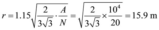
2) Threshold calculation Our algorithm uses the information of the sensing field area and the total number of sensors to calculate the sensing radius and distance threshold dth that match the ideal optimized deployment. The distance threshold is used for deciding the movement of sensors.
As shown in Figure 1, most sensors in the area will have an efficient coverage area which is area E. Assuming that N sensors are deployed in a sensing field with area A, so that each sensor must have an effective coverage of:
 (1)
(1)
The hexagon area E can be written in terms of the sensing radius r as:
 (2)
(2)
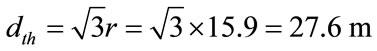
The distance threshold dth and corresponding sensing range r in this case can be calculated as:
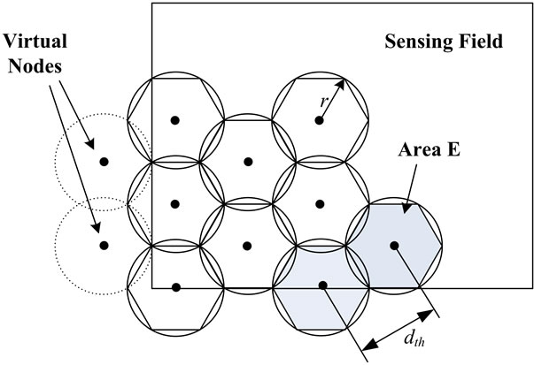
Figure 1. Ideal seamless coverage.
 (3)
(3)
 (4)
(4)
Since the sensors close to either sensing field edge or obstacles will have less efficient coverage, the effective coverage of the sensors inside field must be larger than E. Therefore, the distance threshold and sensing radius must be increased. Here, the sensing radius and distance threshold are increased by 15%.
3) Virtual Nodes For the sensors close to the boundary of sensing field, the algorithm generates virtual nodes along the boundary. The nodes do not exist but their location information will be used in our calculations to prevent sensors from getting too close to the boundary. An example of virtual nodes is shown in Figure 1. Virtual nodes will be used in sensors’ initial relocation and self-healing process.
4) Moving Criteria The goal of our relocation algorithm is to provide a deployment as possible as close to the ideal optimized distribution. It should be pointed out that sensors have no information about the direction of other sensors. Therefore the only information that should be used for relocation is the distance between the sensors. A sensor that needs to move is either too close or too far from other sensors. The moving criteria are described as follows:
Criterion 1: A sensor S needs to move away from other sensors if there is at least one sensor in its communication range of a distance less than 0.9dth;
Criterion 2: A sensor S needs to move closer to other sensors if criterion 1 is not met and no more than 2 sensors are at a distance from S that is less than 1.1dth;
Criterion 3: If criteria 1 or 2 are not met, a sensor does not need to move.
Here, a 10% margin is used so that sensors can achieve a distance close to dth from other sensors.
5) Moving Destination Since there are two criteria 1 and 2 for each sensor, our algorithm will calculate the moving distance for each sensor based on the following equation:
 (5)
(5)
where dj and di are the distance between sensor S and other sensors, and in Criterion 1 only the sensors that are closer than the distance threshold dth are counted, and the total number of such sensors is m1; in Case 2 all the neighbors that sensor S knows are counted and the total number of those sensors is m2.
The relative locations of neighboring sensors are unknown. Therefore, our algorithm chooses randomly the direction of movement. In order to avoid sensors from moving back and forth, a direction control scheme is used. The change of direction between each movement will be less than 90 degrees. Each sensor records the direction α it used in its last movement, and randomly picks another direction within the range of α-90˚ to α + 90˚, for the direction of its next movement. The goal of movement for Criterion 1 is to increase the average distance between sensors, and the goal for Criterion 2 is to decrease the average distance between sensors. Therefore, after sensors randomly choose direction, they will check if going to those directions will meets the goals by moving a short distance to the chosen direction and checking the received signal again. If the random movement does not produce the desired outcome, the sensor moves back and stay the same position in that round.
6) Self-Healing Process Assume a sensor has n1 neighbors it can communicate with after the relocation is finished. After the WSN operates for some time, some sensors lose their functionality and stop working. The sensor now has only n2 neighbors. It will recalculate the distance threshold and sensing range, and then follow the relocation procedure to adjust their locations using the following:
 (6)
(6)
 (7)
(7)
 (8)
(8)
where all subscripts “1” refer to the value before selfhealing process starts, and the subscripts “2” refer to the new calculated value.
7) Obstacle Avoidance When an obstacle blocks the sensors’ relocation path, a sensor has to stop before it hits the obstacle. In the next round the sensor plans its route to move around the obstacle, it can choose to go clockwise or counterclockwise, which depends on which direction satisfies the moving destination calculation. For program simplicity, only regular shape (rectangular) obstacles are considered.
2.4. Relocation Scheme Process
The detailed process of the relocation scheme is as follows:
Step 1: Pre-knowledge installation
• Load sensing range, sensing area and sensors number to sensors memory.
• Load desired round number, set the current round to be Round 1
• Calculate dth, r.
Step 2: Round initialization
• Broadcast and receive “hello” information;
• Calculate the average distance d between sensors by the receiving signal strength;
• Compare the distance condition with the criteria condition and make a moving decision
• Calculate dtravel if needed
• Broadcast moving decision;
• Receive moving decision from other sensors
• Record the number of neighboring sensors that need to move
Step 3: Self-relocation
• If no other sensor nodes declared moving direction choosing process in Set Random time T (conflict avoidance)à
Ø Broadcast “Self-relocation ON”
Ø Choose random direction and move short distance
Ø Broadcast message “Reference node”;
Ø Receive “hello” message respond to message “Reference node”;
Ø Re-calculate average distance d’;
Ø Decide moving direction according to the criteria objective;
Ø Move to destination position and send message “Self-relocation OFF”;
• If a “Self-relocation ON” is received, a sensor will not start the timer T. It will wait until a message “Self-relocation OFF” is received.
• When all sensors finish relocating, this round of the algorithm is finished.
Ø If the round number is equal to maximum allowed round number, go to Step 4.
Ø Otherwise, go to Step 2 and start a new relocation round Step 4: All sensors stop and adjust sensing range to r Step 5: Self-healing l If a sensor detects loss of other sensors, perform self-healing process.
3. Simulation and Analysis
In this simulation, a 100 m by 100 m square sensing field is used. The minimum distance between grid points is 1 m. In this example, we use a sensor network for surveillance that is comprised of motion detector sensors. The sensing range is usually between 18 - 25 m. Therefore, we set the maximum sensing range for our algorithm to be 25 m. Also, the communication range is set to be 55 m, i.e., two times larger than the sensing range in order to guarantee network connectivity. This is also a practical communication range since, for example the Zigbee communication range is 75 m. In this case we did not set the communication range as 75 m because the sensing field is only 100 by 100 m.
3.1. Self-Relocation Algorithm Performance in Non-Obstalce Environment
In the first part, 20 sensors are deployed in the sensing field. Assuming a 15% increase as explained in Section 2.3, the distance threshold and sensing range can be calculated by (3), (4):
 (9)
(9)
 (10)
(10)
Three scenarios are simulated, in which all sensors are randomly deployed initially. In the first scenario, all sensors are deployed in the central 50 by 50 m area; the second scenario has all the sensors randomly deployed in the entire area; and in the third scenario, sensors are split into two groups and deployed near the left and right boundary. The initial coverage for the three scenarios are 50%, 68% and 51%, respectively, when we use r = 15.9 m.
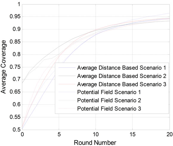
1) Coverage analysis Since the algorithm is based on a random selection of directions, a statistical method is used for the analyzing result. Each scenario is run 10000 times and the desired round number is 20 for all the scenarios. Results are shown in Figure 2.
Figure 2(a) shows how the average coverage increases as the relocation process runs. Specifically, on average 88% coverage is achieved after 10 rounds. Also, the coverage converges to approximately 94% in all scenarios. We also apply the potential field method with the parameters described in [14] in order to compare it with our algorithm. The potential field algorithm provides a converged coverage of 95% after 20 rounds. Therefore, our algorithm and the potential field algorithm converge to approximately the same coverage. Also, our algorithm and the potential field algorithm exhibit the same convergence rate. However, our algorithm does not require the use of GPS or any other self-localization hardware that increase the complexity and cost of the sensor nodes. Also, our algorithm can be used in environments where GPS does not work, such as, indoor, underground, underwater, etc.
Figure 2(b) shows the Cumulative distribution function (CDF) for the coverage achieved after 20 rounds. It is seen that the final coverage after 20 rounds is between 85% and 100% for all three scenarios. It can also be seen that the probability of achieving at least 90% coverage is
 (a)
(a)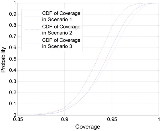 (b)
(b)
Figure 2. Simulation results for self-relocation algorithm: (a) Average coverage vs. round number, (b) Statistical probability of certain coverage after 20 rounds.
larger than 90%. Finally, the standard deviation of the final coverage after 20 rounds for Scenarios 1 and 2 is 2.2%, and for Scenario 3 is 2.6%.
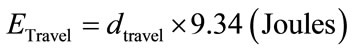
2) Energy analysis For energy analysis, the energy model provided by [15] for its mobile robot is used. According to [15], the energy for a robot platform to move 1 meter is 9.34 Joules when it is in a constant speed at 0.08 m/s, and the energy for the three wheels robot to turn 90 degree is 2.35 Joules. We assume the sensors in the algorithm move in constant speed and turn a constant speed. Therefore, the energy consumed by a sensors’ movement is linearly related to the distance it travels and the angle it turns. Specifically, in each round, the energy consumptions can be divided in two parts:
• Travel: Energy consumed by travel in one direction for each node in each round is calculated by:
 (10)
(10)
•l Direction Changing: In Step 3 in our relocation algorithm, a sensor needs to move a short distance and recalculate the signal strength. After this calculation, a sensor needs to decide to follow that direction or go back to the original position. The energy consumed by the turning process can be calculated by:
 (11)
(11)
where Adiff is the direction difference of the direction before and after the step. If the direction does not meet the requirement for signal strength, the sensor node has to turn back to the original position and the original direction. This is equivalent to turning 360 degrees.
The energy consumed by Potential Field algorithm is also calculated as a comparison. In additional to the energy consumed by travel and direction changing, energy consumed by GPS chip is also included. According to [16], the GPS chip consumes 198 MW. Assuming that sensors move at a speed of 0.08 m/s and neglect the time in between each round for sensors to stop and calculate, so that the GPS consumes  Joules per meter.
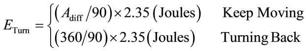
Figure 3 shows the average energy consumption of sensors versus the coverage percentage for our algorithm and the potential field method. It can be seen that the potential field algorithm uses less energy compared to our algorithm. The provided savings in energy consumption are around 25% to 30% depending on the initial deployment. This happens because in the potential field algorithm every sensor knows the location or relative location of all other sensors thereby making better decisions for the directions that the sensors need to move toward. On the contract, our algorithm consumes more energy when it turns back and forth. However, our algorithm does not require that sensors know others location or transmit their location information to other sensors. This can provide significant savings in terms of hardware cost since no GPS hardware is required.
Figure 3. Simulation results for relationship between average coverage and energy consumption.
3.2. Simulation for Self-Healing Algorithm
After the execution of the self-relocation algorithm, we randomly choose five sensors to die. The initial deployment for our self-healing simulation is shown in Figure 4. The 5 nodes without coverage are assumed dead.
The simulation results are shown in Figure 5. This simulation is also run 10000 times. Figure 6 shows the average, best case and worst case coverage. After the sensors have died, only 80% coverage is provided. However, our algorithm increases the coverage by increasing the sensing range of each sensor. After the first round, the coverage ratio increases slowly because the sensors need to move slowly toward the areas that are not covered. After 20 rounds, our algorithm achieves an average coverage of 93%. In this case, the average sensing range of the sensors is approximately 18.3 m thereby providing 26.8% energy savings compared to the case where the sensors use their maximum sensing range of 25 meters. The average traveled distance in the self-healing process is around 7.5 m.
Figure 6 shows one sample simulation for our selfhealing algorithm. The moving processes of all the sensors are shown. Blue dots are the initial position of the sensors, and the red stars are final positions. Figure 6
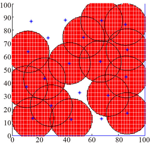
Figure 4. 5 sensors die in originally 20 sensors field.
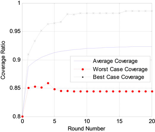
Figure 5. Coverage result for self-healing algorithm.
also shows the final uncovered area in red. It can be seen that in the left up corner where three sensors died, other sensors have not move enough to completely cover this area. However, for the other two places, where only one sensor has died (middle and bottom of the sensing field), the self-healing algorithm provides almost complete coverage of the area that the dead sensors covered.
3.3. Self-Relocation Algorithm Performance in Environment with Obstacles
In this part, two obstacles are placed in the sensing field and 20 sensors are in the middle part of the sensing field which is shown in Figure 7. Due to the appearance of obstacle, 10% increase in sensing radius is applied. The initial coverage is 19% with the sensing radius of 17.5.
Figure 8 shows the CDF of the final coverage after 20 rounds. In fact, 90% coverage is achieved on average after 20 rounds. The standard deviation of the final coverage is 3%. Since the obstacles occupy 150 m2 in total, the maximum coverage cannot exceed 98.5%.
4. Conclusion and Future Work
In this paper, we developed a self-relocation and selfhealing algorithm based on average distance. The sensors only need to know the approximate area of the sensing
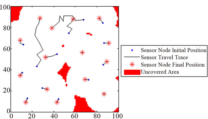
Figure 6. A sample simulation of self-healing process.
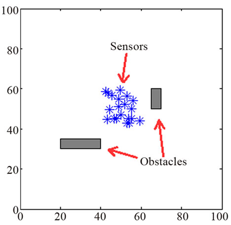
Figure 7. Initial deployment in field with two obstacle.
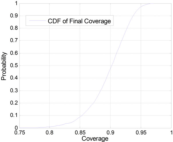
Figure 8. Statisitcal coverage result in self-relocation algorithm with obstacles’.
field and the total number of sensors before they are deployed. The sensing range of each sensor is adjusted to reduce the redundancy and provide energy savings. No geo-location or relative location knowledge is needed thereby providing significant savings for each node since GPS hardware is not required. However, the tradeoff is that the sensors nodes have to consume more energy to achieve certain percentage of coverage compared to the algorithm using GPS devices. The algorithm works for both environments with or without the appearance of obstacles. The disadvantage of our algorithm is that the direction movement is random and not always the best direction thereby resulting in larger traveled distance. Our algorithm is suitable for emergency surveillance where sensors don not have GPS devices and localize themselves by cooperation with other sensors only when emergencies or trigger events occur in their sensing range.
REFERENCES
- V. Potdar, A. Sharif and E. Chang, “Wireless Sensor Networks: A Survey,” Advanced Information Networking and Applications Workshops, Bradford, 26-29 May 2009, pp. 636-641.
- T. H. Arampatzis, J. Lygeros and S. Manesis, “A Survey of Applications of Wireless Sensors and Wireless Sensor Networks,” Proceedings of the 2005 IEEE International Symposium on Mediterrean Conference on Control and Automation, Limassol, 27-29 June 2005, pp. 719-724.
- J. Chen and C. Li, “Coverage Optimization Based on Improved NSGA-II in Wireless Sensor Network,” IEEE International Conference on Integration Technology (ICIT), Shenzhen, 20-24 March 2007, pp. 614-618.
- X. Wang, S. Wang and D. W. Bi, “Dynamic Sensor Nodes Selection Strategy for Wireless Sensor Networks,” 7th International Symposium on Communications and Information Technologie (ISCIT), Sydney, 16-19 October 2007, pp. 1137-1142.
- J. Weck, “Layout Optimization for a Wireless Sensor Network Using a Multi-Objective Genetic Algorithm,” IEEE 59th Vehicular Technology Conference, Milan, Vol. 5, 2004, pp. 2466-2470.
- L.-C. Wei, C.-W. Kang and J.-H. Chen, “A Force-Driven Evolutionary Approach for Multi-Objective 3D Differentiated Sensor Network Deployment,” IEEE 6th International Conference on Mobile Adhoc and Sensor Systems (MASS), Macau, 12-15 October 2009, pp. 983-988.
- A. Howard, M. Mataric and G. Sukhatme, “Mobile Sensor Network Deployment Using Potential Fields: A Distributed, Scalable Solution to the Area Coverage Problem,” The 6th Internotional Symposium on Distributed Autmomous Robotics System, Fukuoka, 25-27 June 2002, pp. 299-308.
- Yi. Zou and K. Chakrabarty, “Sensor Deployment and Target Localization Based on Virtual Forces,” IEEE Societies Twenty-Second Annual Joint Conference of the IEEE Computer and Communications (INFOCOM), San Fransisco, 1-3 April 2003, pp. 1293-1303.
- M. R. Pac, A. M. Erkmen and I. Erkmen, “Scalable SelfDeployment of Mobile Sensor Networks: A Fluid Dynamics Approach,” Proceedings of IEEE International Conference on Intelligent Robots and Systems (RSJ), Beijing, 9-15 October 2006, pp. 1446-1451.
- R.-S. Chang and S.-H. Wang, “Self-Deployment by Density Control in Sensor Networks,” IEEE Transactions on Vehicular Technology, Vol. 57, No. 3, 2008, pp 1745-1755. doi: 10.1109/TVT.2007.907279
- G. Wang, G. H. Cao, T. F. Porta and W. S. Zhang, “Sensor Relocation in Mobile Sensor Networks,” IEEE Societies 24th Annual Joint Conference of the IEEE Computer and Communications, Miami, 2005, pp. 2302-2312.
- M. Cardei, J. Wu, M. M. Lu and M. O. Pervaiz, “Maximum Network Lifetime in Wireless Sensor Networks with Adjustable Sensing Ranges,” IEEE International Conference on Wireless and Mobile Computing, Networking and Communications, Montreal, 22-24 August 2005, pp. 438-445.
- G. Wang, G. H. Cao and T. F. Porta, “Movement-Assisted Sensor Deployment,” IEEE Transactions on Mobile Computing, Vol. 5, No. 6, 2006, pp. 640-652. doi:10.1109/TMC.2006.80
- W. H. Sheng, G. Tewolde and S. Ci, “Micro Mobile Robots in Active Sensor Networks: Closing the Loop,” Proceedings of IEEE International Conference on Intelligent Robots and Systems (RSJ), Beijing, 9-15 October 2006, pp. 1440-1445.
- Y. G. Mei, Y.-H. Lu, Y. C. Hu and C. S. G. Lee, “Energy-Efficient Motion Planning for Mobile Robots,” Proceedings of IEEE International Conference on Robotics and Automation (ICRA), New Orleans, 25 April-1 May 2004, pp. 4344-4349.
- M. K. Stojcev, M. R. Kosanovic and L. R. Golubovic, “Power Management and Energy Harvesting Techniques for Wireless Sensor Nodes,” 9th International Conference on Telecommunication in Modern Satellite, Cable, and Broadcasting Services, 7-9 October 2009, pp. 65-72.
- CC4000GPSEM, “CC4000 GPS Module Kit,” Texas Instruments. http://www.ti.com/tool/cc4000gpsem