Wireless Sensor Network
Vol.4 No.9(2012), Article ID:22511,8 pages DOI:10.4236/wsn.2012.49031
Queuing Management in Wireless Sensor Networks for QoS Measurement
1Institute of Cybernetics, Baku, Azerbaijan
2Qafqaz University, Baku, Azerbaijan
Email: agassi.melikov@rambler.ru, anar.rustemov@gmail.com
Received July 6, 2012; revised August 10, 2012; accepted August 20, 2012
Keywords: Wireless Sensor Networks; Buffer; Queuing Theory; QoS; Multimedia Data
ABSTRACT
Data transmission in multimedia WSNs are required high bandwidth and reliable transfer because of large amount of data size. However, some applications of WSNs are required high quality. In this context, main factor in quality of services (QoS) metrics in WSNs becomes longevity of the network and high quality. In sensor nodes, choosing relevant transceiver and microcontroller components plays important role in assembling sensor devices, in which data controls should be designed so that packet loss is minimized. Available QoS metrics based on queuing/buffer management in wired and other wireless networks don’t applicable in WSNs because of its unique characteristics. In this paper the simplest model of QoS model-bufferless system were proposed. In the proposed model, measurement of the probability of blocking of the arrival packets was suggested by using queuing theory in order to increase QoS. Given probability of blocking (PB) illustrates clear picture how system specification should be chosen so that blocking state would be minimized.
1. Introduction
Wireless Sensor Networks (WSNs) are a widely investigated area in the last decades. WSNs consist of tiny, limited resourced, low-cost and wirelessly connected devices called sensor node [1]. The sensor nodes connect with each other on the basis of multi-hop network. The nodes are embedded with the sensor boards to sense the environmental phenomenon and are scattered over the unattended areas in order to collect sensing data and send them to the destination node called sink. As, in general, the sensor nodes aren’t reusable, it is assembled of lowcost and off-the-shelf devices in order to keep its cost cheaper. Considering the fact that the nodes have resource constraints, they are able to perform low tasks that require less computation. Furthermore the batteries of the nodes are irreplaceable, which in term create many challenges in the node and network design. As a main problem-energy consumption should be taken into account in all the research topics related to WSNs, such as network design and protocols, network management, error correction and etc. Each sensor node performs environmental monitoring and simultaneously plays a role of router. It sends gathered data to the sink through mediate nodes and receives the packet coming from the neighbor nodes. A battery-depleted or failed nodes change network topology and directly or indirectly shorten the life of the sensor networks [2].
Because of limited resource, the sensor nodes have application-specific characteristics. Namely, the software programs in the nodes are designed based on the environmental phenomenon in order to consume less energy. Another factor that affects negatively energy consumption is data routing protocol. The major factor in designing of routing protocols is to do less computation in order to conserve energy. Therefore transmission error checking, path selection and etc. should be chosen so that it would be aimed to the purpose given above [3].
In traditional sensor networks a size of delivered packets is quite small to be delivered from the source node to the destination node. In the case of multimedia data where a size is measured in megabyte (Mbytes), it is a big challenge to transfer the data. The bigger the data, the more computation and energy are required to deliver the packets.
Therefore wireless multimedia sensor networks (WMSNs) are required different routing protocols, modified sensor nodes with high speed processors that could process the multimedia data. In WMSNs energy consumption still remains the main problem. As we increase hardware specifications, more energy will be consumed and vice versa. One of the ways to prolong the life of nodes is to add additional power supply such as a solar cell. However, it will increase the cost of the sensor nodes and therefore will squeeze the application areas [4]. Regardless of the challenges mentioned above, there should be trade-off between energy consumption and resource utilization. However, service time for each arrival packets increases as the size expands, therefore, number of packets waiting in queue in the buffer are swelled. The loss of some video and voice packets might not seriously affect overall data in destination, so that remaining packet can convey the necessary message to the listener. In the case of loss of image packet, it is difficult to rearrange whole frame in order to get original picture back. In this paper we gave Quality of Service measurement by analyzing the packets in the queue by using Queueing Theory.
2. System Overview of Multimedia Wireless Sensor Networks (WSNs)
A wireless sensor nodes consist of several sensor nodes wirelessly connected with each other. Each sensor nodes are composed of processor unit (CPUs, microcontrollers), memories (random access memory (RAM) and low-sized flash memory), power supply, a RF transceivers (to connect with other sensor nodes) and sensor board (to sense the environmental process) [5]. Sensor nodes can be used in different areas such as event detection, location sensing and etc. Each node is self-organized and based on the routing protocol they communicate with neighbor nodes to deliver gathered data to the destination nodes called a sink. A sink is a gateway between WSNs and internet/ intranet. As a sink has continuous power supply, it can connect and support all kinds of network structure and architecture. System administrators communicate with sensor through the sink. State-of-the-art sensor nodes have ability to analyze data and deliver relevant part of them; where in turn perform very less processing computation. Considering fact that sensor nodes spend most of their energy on transmitting and receiving data, this ability of the nodes is a very important factor to prolong life of the sensor networks [6]. Because of hardware source and power limitations, sensor nodes cannot work with traffic classes such as video, voice, picture and stream data effectively. Currently available Complimentary Metal Oxide Semiconductor (CMOS) cameras that are small in size and image obtained from them are of low quality make the usage of multimedia data in WSNs very efficient and practical. However with sufficient image quality, multimedia data transfer requires incredibly high bandwidth. In this circumstance the main purpose in transferring multimedia data over the nodes is to prolong the lifetime of the sensor network. Unlike traditional WSNs where data size is quite small, multimedia WSNs require totally different network design including routing protocol, encoding/decoding, path selection and etc. In addition, one of the priority issues in multimedia communication is to minimize the data loss that occurs during the queue at MAC layer. Therefore Quality of Service (QoS) metrics for multimedia WSNs significantly differ from the one for conventional WSNs. More detail about QoS in multimedia WSNs we will talk in the following sections. Furthermore there are several factors that influence multimedia communication between sensor nodes. These factors are given in the next sub topics.
2.1. Hardware Architecture
Sensor nodes in multimedia WSNs are embedded with low-cost video cameras or sound recorders as well as sensor boards. When sensors act in detection of intruders or any environmental phenomenon then video cameras or sound recorders are activated. For data generation, operation and communication additional power supplies are necessary to keep the lifetime of the nodes long [7]. Depending on an application of multimedia WSNs the network topology is changed based on the network architecture, where the changes should serve for reducing the multimedia data. It is fact that the bigger queue in each node, the bigger the probability of data loss.
2.2. Processor
Up-to-date microcontroller used in WSNs is a small computer on a single integrated circuit containing a processor core, memory, and programmable I/O peripherals. Unlike microprocessors used personal computers, laptops and etc., microcontrollers are designed for embedded applications. There are several key components in selection of microcontrollers that are essential for designing of sensor nodes, such as power, voltage, cost and support for other external devices. As a main problem, energy must be less consumed during the installation and implantation. Therefore selection of relevant microcontroller family should be carefully determined. To determine trade-off between energy consumption and computation is the most important metric. Peak power consumption might not always be suitable for the task specified on curtain applications. Microcontrollers in sensor nodes consume subtle energy during the sleep mode. During the sleep mode CPU stops its work and shifts to the save mode where very less energy is needed for computation. Furthermore, the processor has to be awake in order to maintain the systems memory and time synchronization [8,9]. Figure 1 is illustrated basic hardware architecture of a sensor node. In the next topics we will analyze processing unit where the buffer is placed in order to increase Quality of Services.
2.3. Protocol Stack and Queuing Management
In this paper we mainly focus on analyzing of queue at MAC layer in order to determine some QoS metrics. However we will touch other layers briefly, but MAC and Physical Layer detailed. Although there are different standards for WSNs, such as WirelessHART, ISA100, IEEE 1451, ZigBee/802.15.4, common accepted protocol stack is determined in five levels (Figure 2).
A. Application Layer: It is the layer that provides us interface to connect to the platform in order to run deployed software depending on experiment type. Moreover, all the services, tasks and other background applications used in the networking connectivity, data analyzing and etc. run at this layer.
B. Transport layer: It controls data flow from the application layer to network layer. Segmentation of data and reassembling arrival segments are generated in this layer.
C. Network layer: This layer is responsible for routing schema, path selection. In addition, addressing, encapsulation and decapsulation are taken place in this layer.
D. Data Link layer: is the layer that makes link between software and medium. Data Link layer are divided into two sub-layers: 1) Upper sub layer—Logical Link Control (LLC) layer and 2) Lower layer—Medium Access Control (MAC) layer.
LLC Layer acts as an interface between the MAC layer and the network layer. Its main responsibilities to provide services to the network layer protocols and particularly to control frame synchronization, flow control and error check.
MAC Layer determines the media access controlling on hardware devices and provides data analyzing based on physical signaling requirements of the medium. Since medium in WSNs is made of wireless technologies, enhancing the radio design and effective MAC protocols that will decrease power consumption in a radio is a main channeling issue in protocol design in MAC sub layer. Functionalities of MAC protocol are changed depending on the Network layer requirements, hardware specifications and network topologies [3] (see Figure 2).
As proposed in [10] MAC layer QoS can be classified mainly into channel assess policies, scheduling and buffer management and error control. In this paper we addressed buffering problem in MAC layer in order to improve QoS in data transmission.
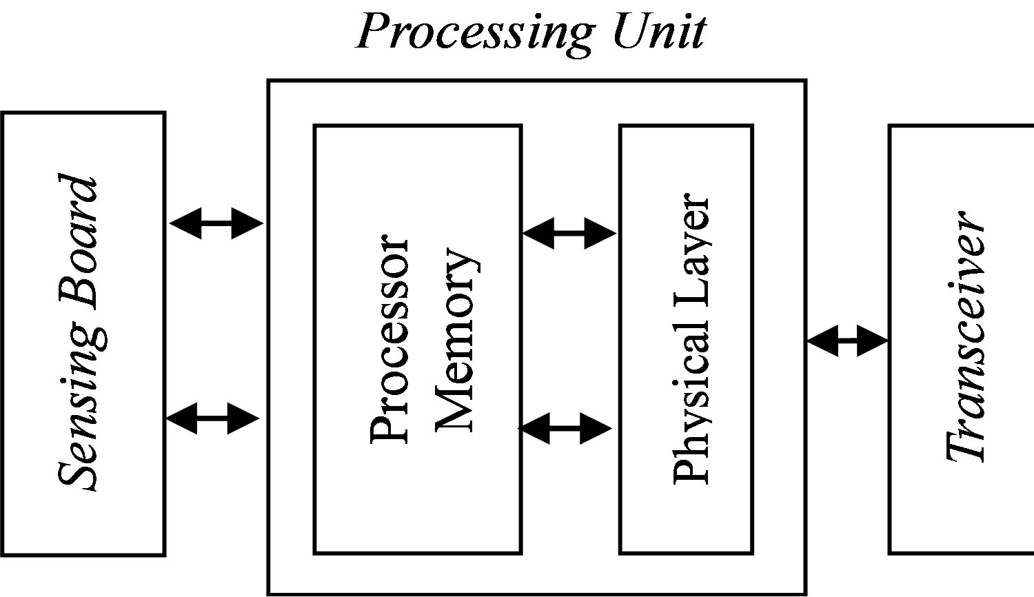
Figure 1. Basic hardware architecture of a sensor node.
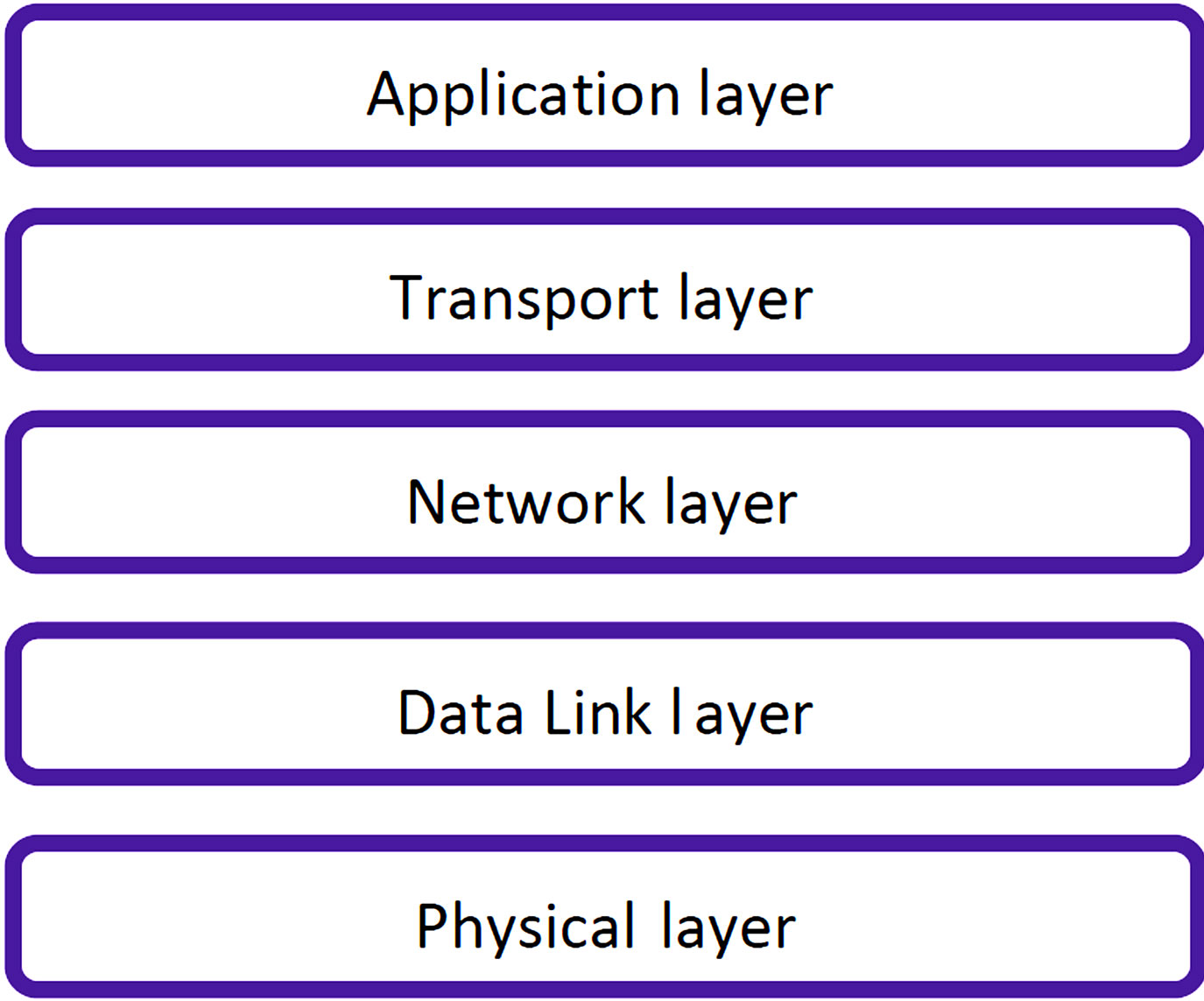
Figure 2. The WSNs protocol stack.
E. Physical layer: This layer directly converts coming frames from MAC layer to wireless signal. Transmitted bits go through encoding process before sending via the media. Following Physical layer elements are necessary to transfer the frames: a) the physical media and connectors, b) encoding and decoding mechanism, c) transmitters and receiver circuitry embedded on sensor nodes.
In this paper we took Physical layer and MAC sub layer together as one “service point” and remaining layers together as second “service point” to determine QoS metric based on the data queue stored in MAC layer.
As we mentioned above big size of multimedia traffic and low computational ability of the sensor nodes result in buffer overflow at the receiver. Since there are significantly different between multimedia WSNs and other wireless networks, such as ad-hoc, mobile, in terms of traffics classes and their size, queueing process and scheduling context of them in the MAC layer will be different [11]. Queueing process in the MAC layer has been extensively researched and several schemes with varying levels of complexity were proposed. Queueing process directly related to the energy consumption. So that data packet loss because of buffer overload leads to retransmission of the same packets several times, which in turn consume additional energy.
To show an importance of queueing model in multimedia WSNs, we illustrated the big picture of the queueing process in Figure 3. As shown in the figure, Processor Memory is divided into logical part in order to picture the work flow distribution from the perspective of the protocol stack.
3. Motivation and Research Framework
As we mentioned above, in WSNs all QoS metrics should lead to less energy consumption. In the proposed model, we focused on buffering mechanism in the MAC sub layer in order to prevent the loss of arrival packets, therefore, to minimize retransmission which in turn results in less power consumption. In order to reduce the blocking probability of arrival packet with intensity λ, we
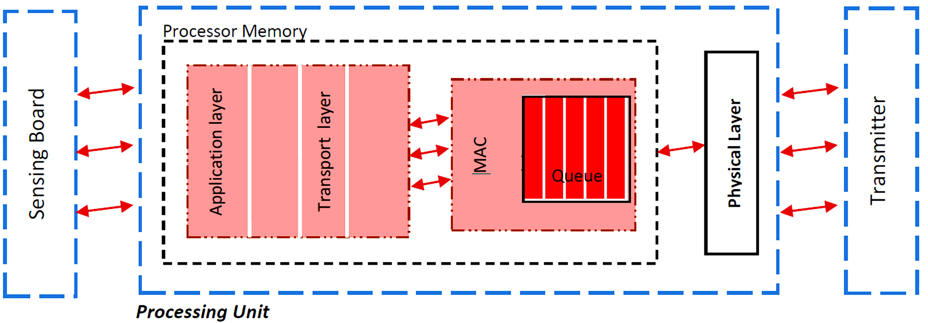
Figure 3. Queueing process in the processor memory.
divided the processor memory (see Figure 3) into two parts as separate service points. The MAC sub layer was determined as one server with service intensity μ1 and remaining network layers were taken as a one server with service intensity μ2 (see Figure 4). Arrival packets enter the MAC sub layer through the physical medium (physical layer) and waits in the queue if the system is busy.
For simplicity and as a first case, we took bufferless system and showed the QoS metric on arrival data intensity. Based on our result it is possible to determine rate of transmission/receiving and the specification of microcontrollers. In our future works we will consider the buffer and traffic types in our model.
In Figure 5 is illustrated the state diagram based on the state spaces given as follows: (0,0), (1,0), (0,1), (1,1), b (block). The state (0,0) means the system is empty and there isn’t any packet received. When the first server receives a packet and serves it, while the second server is idle, the system goes to (1,0) state. If the packet is forwarded to the second server to serve, then the system state becomes (0,1). In this state the first server must be idle. Other vise the system state will be in (1,1) state. Namely both of the servers will be busy. The state b (blocking) happens when the first server is finished its task, but the second server is still in working regime. If the first serve is not idle, then arrival packet will be dropped.
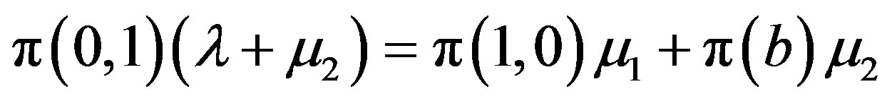
Let p(x) denote steady state probability of state x. State probabilities for given model are satisfies the following balance equations:
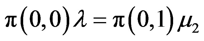 (1)
(1)
 (2)
(2)
 (3)
(3)
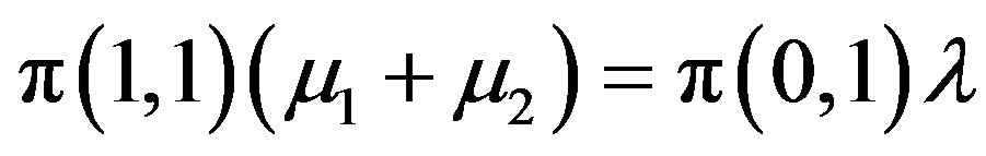 (4)
(4)
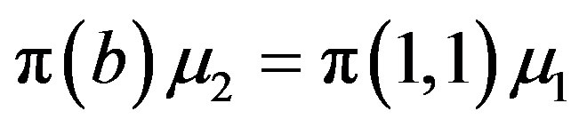 (5)
(5)
Normalizing condition for the given model is:
 (6)
(6)
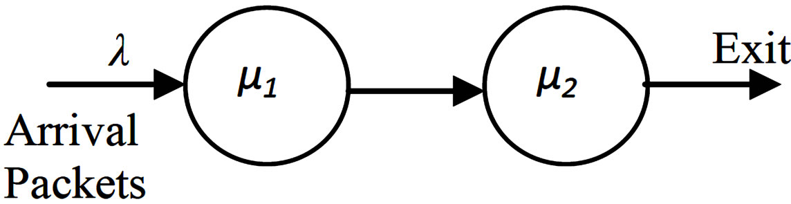
Figure 4. Structure of queueing process.
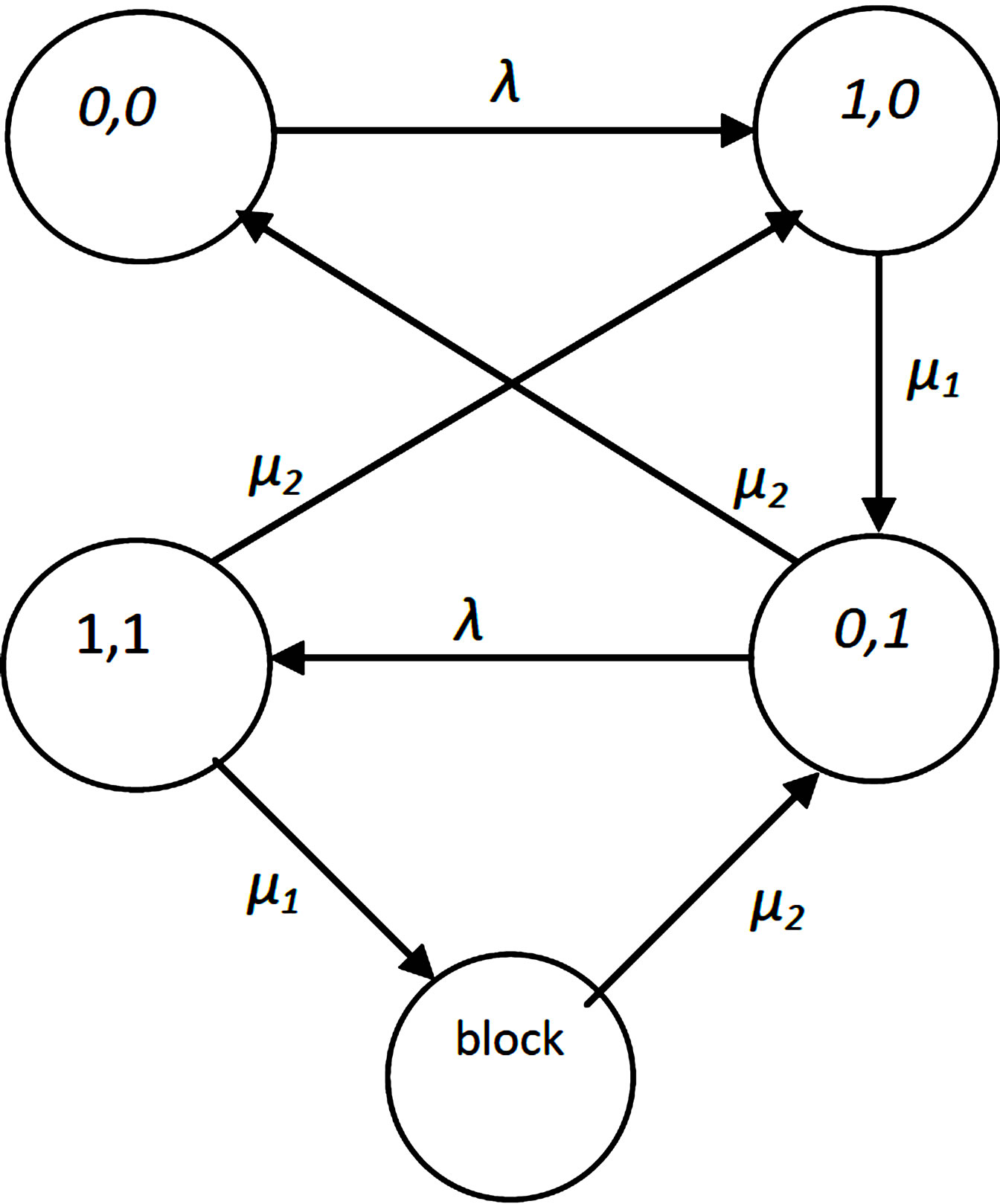
Figure 5. The state diagram of system.
For analyzing the model we took two cases a) general case, where  and b) special case, where
 .
.
In general case, computation speed of the CPU should be faster than receiving and a service speed at the MAC layer. Other vice, packets flowing from the MAC layer to the up layers either will be loss or should wait in the queue. Since in our model we consider bufferless system in each part, we can propose that . Nevertheless our model is designed to all cases under the condition of
 .
.
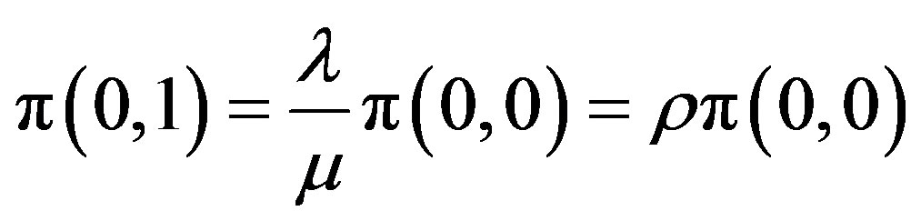
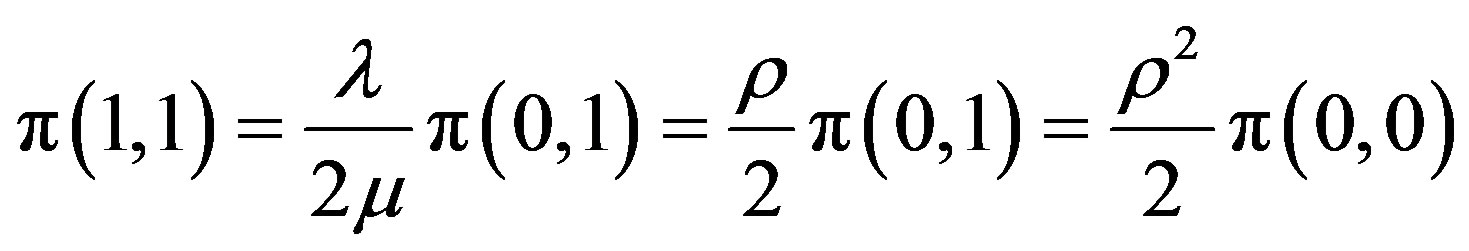
Using mathematical calculation we can calculate the state probabilities (π) as follow. From (1) we can get calculation of π(0,1) as given in (7). By applying (7) to (4), state probabilities π(1,1) is derived as (8).
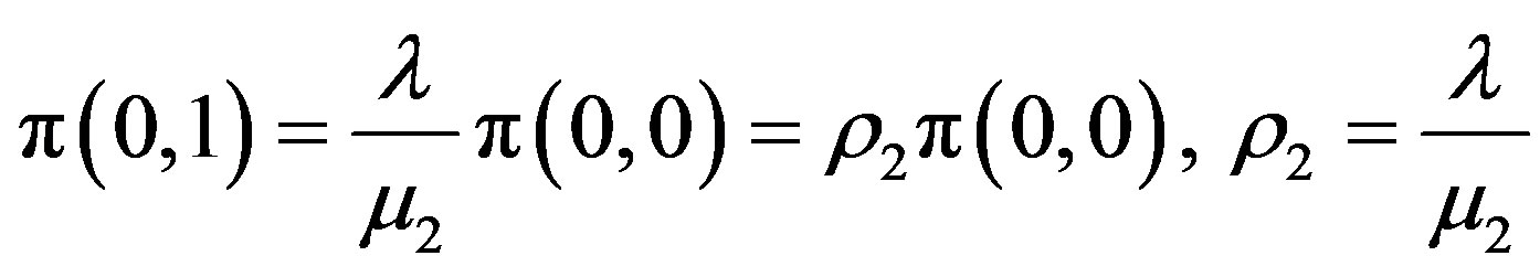 (7)
(7)
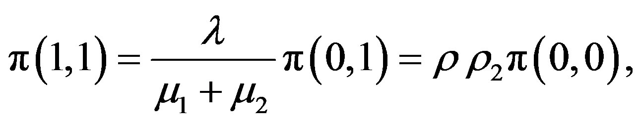 (8)
(8)
where 
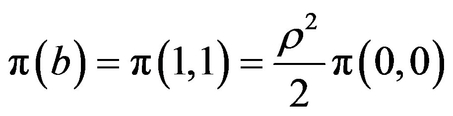
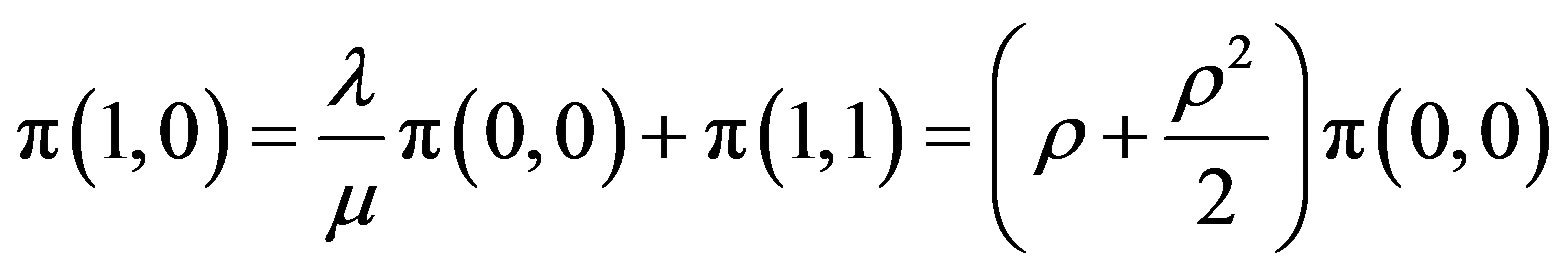
Furthermore, considering (8) in (5), measurement of π(b) can be given as (9). Calculation of state probability π(1,0) can be derived by substituting (8) in (2).
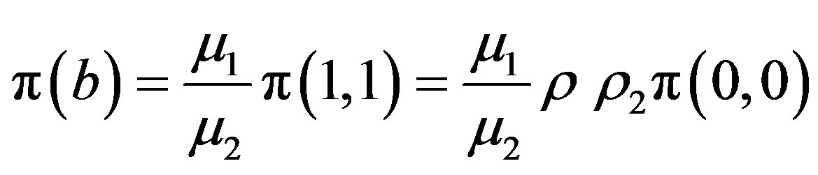 (9)
(9)
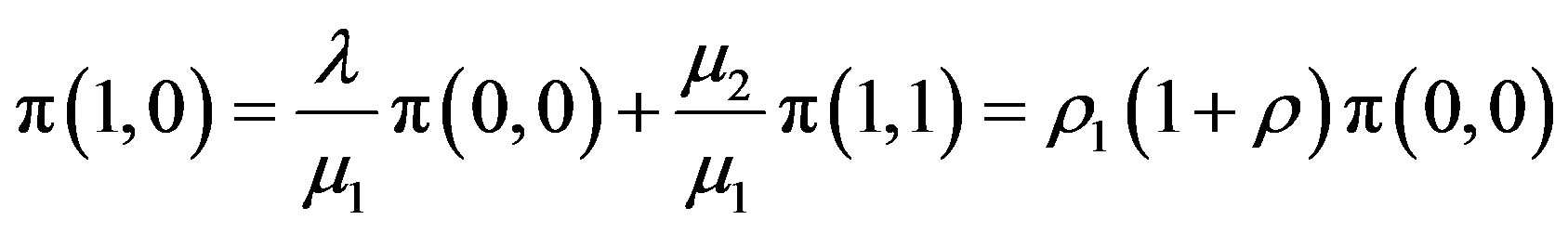 (10)
(10)
where 
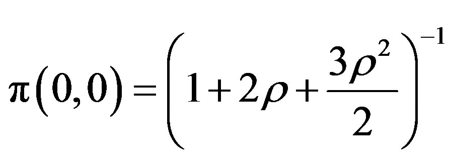
Finally from normalizing condition (6) we get measurement of π(0,0):
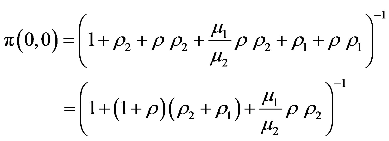 (11)
(11)
Here we are interested in the probability of blocking as a QoS Metric. In the proposed model the probability of blocking (PB) happens when the first server is busy and in the state of blocking. Eventually, we can calculate PB as below:
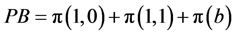 (12)
(12)
In special case, we analyzed the case where μ1 = μ2,
 By implementation simple substitution in (7)(12), the state probabilities can be given as follow:
 (13)
(13)
 (14)
(14)
 (15)
(15)
 (16)
(16)
 (17)
(17)
The probability of blocking system (PB) will be measured as below:
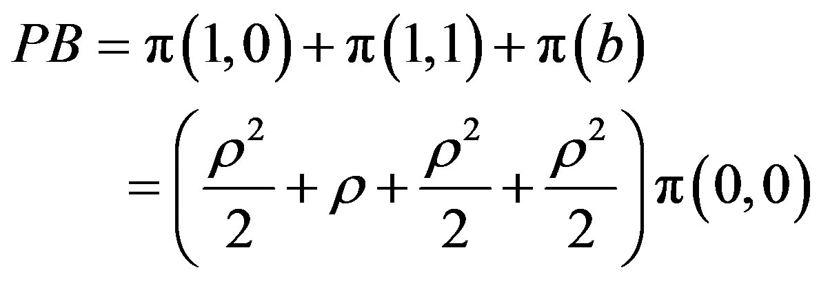 (18)
(18)
Based on the exact formulas of state probabilities, we did numerical analyses for both cases.
4. Numerical Results
Since we study buferless system in our model, we were only interested in Probability of Blocking (PB) of the arrival packets. Furthermore, for simplicity we took the nature of all the traffic classes (video, sound, picture and streaming) as a single multimedia class. In each traffic class a size of the packet is quite big to transfer through the sensor networks. Minimization of the probability of data loss is a very important factor for the WSNs. Some results are shown in Figures 6-9. The curves coincide with all theoretical expectations. In both cases relationship between PB and μ1, μ2, λ are deeply analyzed. One of the main purposes of the QoS metrics is to minimize the blocking probability of the arrival packets. Probability of blocking is negatively related with the arrival intensity λ. Indeed, as λ gets big, a number of packets to be served by the server 1 also increase. In Figure 6 is given their relationship in different values of μ1 and μ2. Furthermore, this behavior acts the same when service intensities of the server 1 and 2 are equal (μ1 = μ2). The best option to get less blocking probability is to maximize μ1 if μ2 is fixed. As given in the Figure 6 PB is bigger in μ1 = 15, and less in μ1 = 25.
To get a clear picture of dependence we set μ1 equal to μ2 as a special case. As shown in Table 1, PB increases by decreasing rate as μ goes up. Dependence of PB from μ is given in Figures 7-9. Obviously, a blocking probability should be positively related to service intensities μ1 and μ2. The bigger service intensity is, the bigger a number of packets to be served; therefore a number of blocked packets become much less. It is clear from the
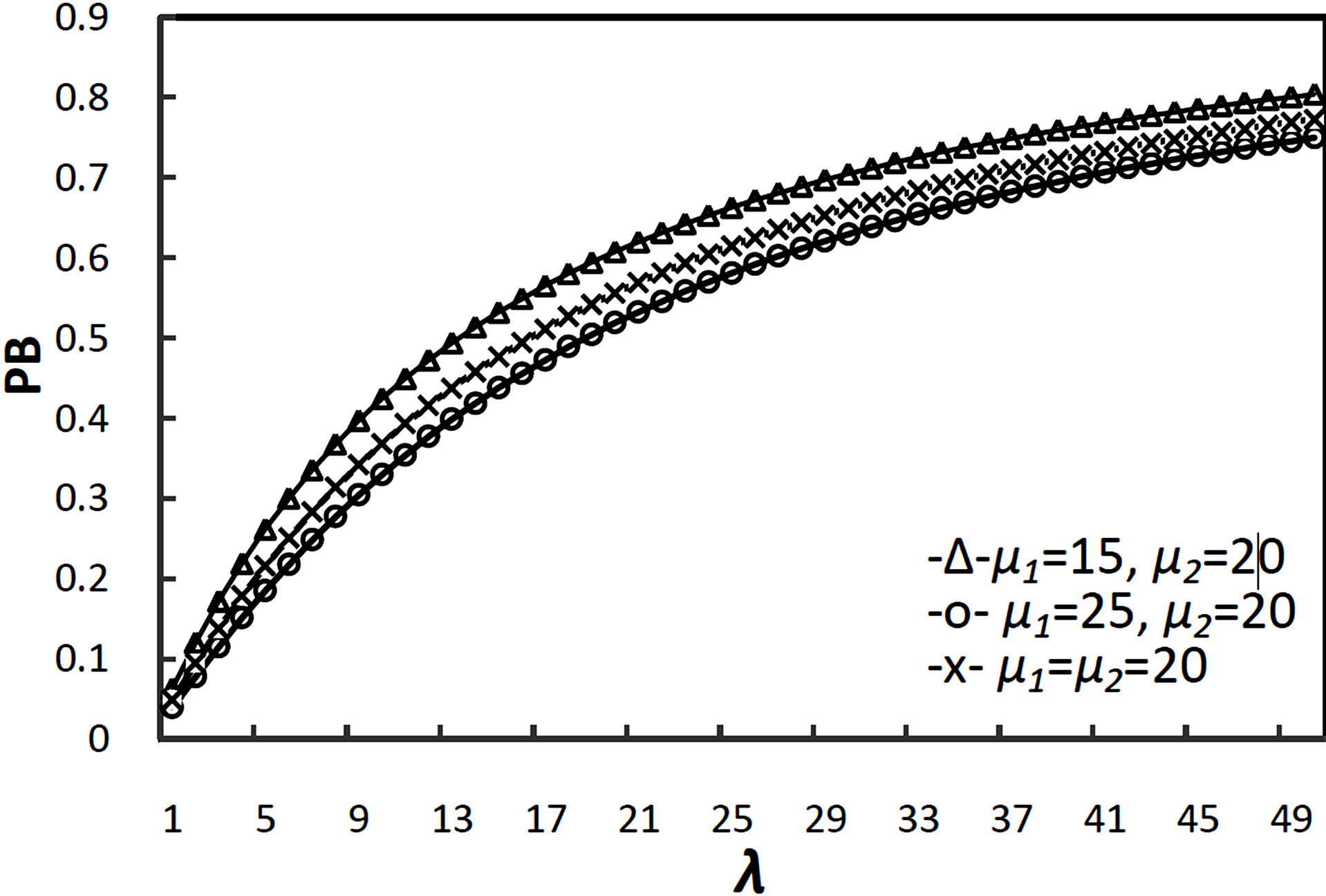
Figure 6. Blocking probability of arrival packets versus λ.
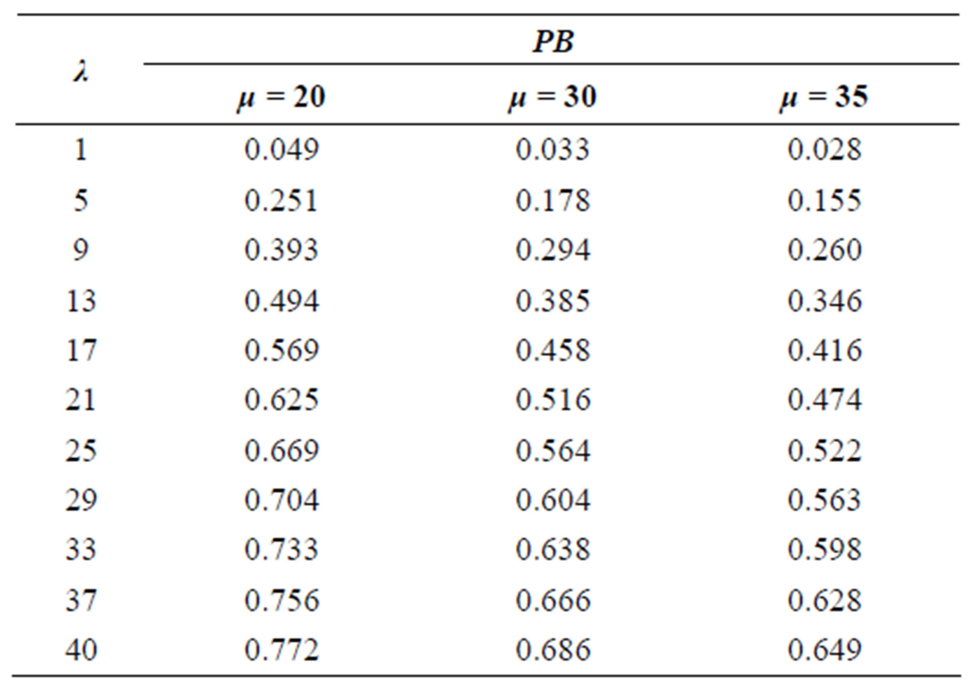
Table 1. Comparison of Probability of Blocking (PB) in different values of μ (μ1 = μ2 = μ) depending on λ.
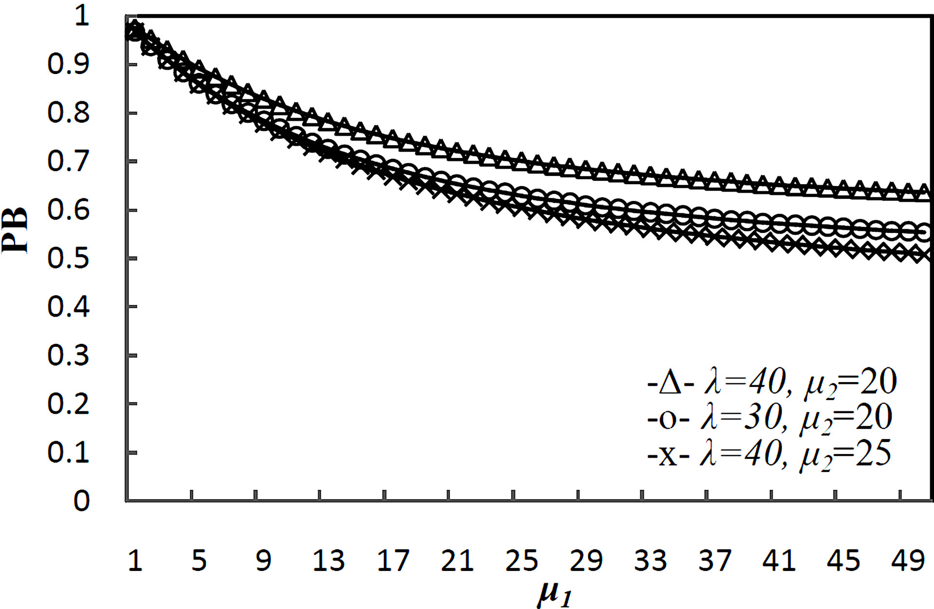
Figure 7. Blocking probability of arrival packets versus μ1.
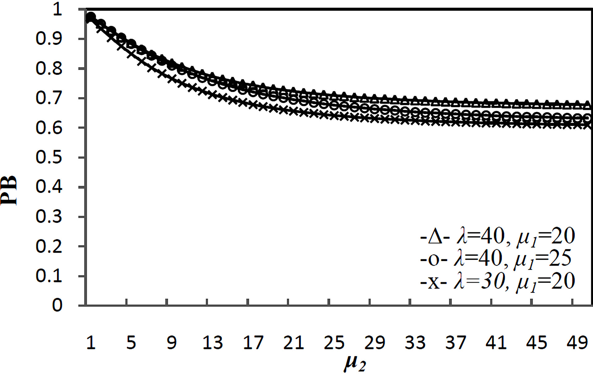
Figure 8. Blocking probability of arrival packets versus μ2.
Figures 7 and 8 that a probability of blocking is decreasing as service intensities increase. In practice the case of μ1 ≥ μ2 makes sense, other vise state probability of b (blocking) will be increased, that will result in increase in queue at the first server. In Figure 7 the blocking probabilities of the cases λ = 40, μ2 = 20 and λ = 40, μ2 = 25 are given respectively. At the beginning values of PB in both cases are almost the same. However toward the end PB of the second case where μ2 = 25 is getting much bigger, which satisfies our hypothesis. The same behavior can be seen in Figure 8—relation of PB versus μ2, so that the best result is given in the case of μ1 = 25, where λ = 40. Basically higher arrival intensity makes it difficult to serve the entire packet by the server. As shown in Figure 9, PB get smaller values depending on μ when λ = 20 and the highest when λ = 35. Hypothetically, it satisfies the expected results.
To get a clear picture of dependence we set μ1 equal to μ2 as a special case. As shown in Table 1, PB increases by decreasing rate as μ goes up. Dependence of PB from μ is given in Figures 7-9. Obviously, a blocking probability should be positively related to service intensities μ1 and μ2. The bigger service intensity is, the bigger a number of packets to be served; therefore a number of blocked packets become much less. It is clear from the Figures 7 and 8 that a probability of blocking is decreasing as service intensities increase. In practice the case of μ1 ≥ μ2 makes sense, other vise state probability of b (blocking) will be increased, that will result in increase in queue at the first server. In Figure 7 the blocking probabilities of the cases λ = 40, μ2 = 20 and λ = 40, μ2 = 25 are given respectively. At the beginning values of PB in both cases are almost the same. However toward the end PB of the second case where μ2 = 25 is getting much bigger, which satisfies our hypothesis. The same behavior can be seen in Figure 8—relation of PB versus μ2, so that the best result is given in the case of μ1 = 25, where λ = 40. Basically higher arrival intensity makes it difficult to serve the entire packet by the server. As shown in Figure 9, PB get smaller values depending on μ when λ = 20 and the highest when λ = 35. Hypothetically, it satisfies the expected results.
Since selection of relevant specifications of microcontrollers is important, trade-off between service intensities of first and second servers should be considered as main factor affecting energy consumption. In this regards we analyzed relation between blocking probability and ratio of μ1 and μ2 (μ1/μ2) (Figure 10). We took curves in three
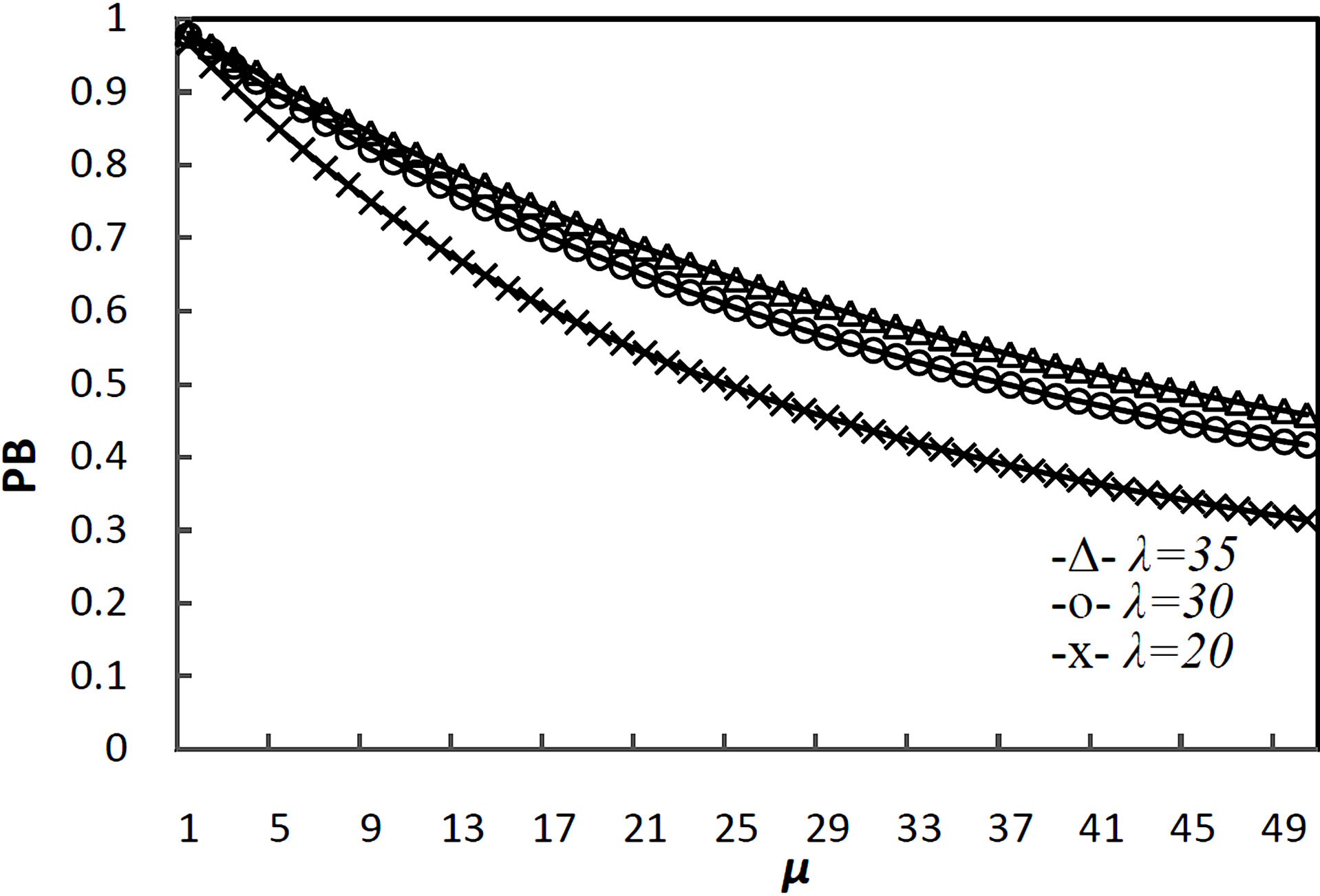
Figure 9. Blocking probability of arrival packets versus μ.
different values of λ (λ = 50, λ = 70, λ = 100) and increased the values of μ1 and μ2 based on the ratios as 0.25, 0.5, 0.75, ···, 5. As given in the graph, this relationship implies that there is always a blocking probability in the given model and the best ratio between μ1 and μ2 is the minimum one, namely the best choice is when μ1 is less than μ2 as much as technically possible. Therefore in selection of relevant microcontroller we should pick the one in which service intensity of the first server is less than second one or other vise in which service intensity of the second server is bigger than first one. The case of higher blocking probability when ratio of μ1/μ2 is bigger is reasonable, so that if the first server sends the packets with high intensity to the second server with low service intensity, then the second one cannot serve properly and therefore it will lead to data loss in the first server.
Theoretically is known that the bigger the arrival intensity, the bigger data lost or the probability of blocking if to keep other parameters as constant. This phenomenon is obvious in Figure 10 too, so that in the case of λ = 50 the probability of blocking is having the lowest values; however in the case of λ = 100 it has the biggest values.
Based on the algorithm proposed above for measurement the blocking probability PB, it is possible to give optimization solutions for these quantities of μ1 and μ2. Since PB is a monotonically decreasing function of μ1 and μ2, we can propose the following minimizing problem for the given model:
1) Find the minimum  subject to PB ≤ ε1, where ε1, λ, μ2 is fixed and given in advance, i.e.
 (19)
(19)
 (20)
(20)
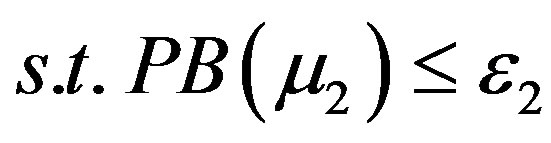
2) Find the minimum  subject to PB ≤ ε2, where ε2, λ, μ1 is fixed and given in advance, i.e.
 (21)
(21)
 (22)
(22)
By using monotonic property of function PB, we can increase the values of μ1 and μ2 step by step till they satisfy (20) and (22) respectively. Satisfied values are the minimum values of  and
and  respectively. The results of a solution of the optimization problems (19)-(22) are given in Tables 2 and 3 respectively. A symbol Ø given in the tables means that solution for the problem are achieved at very high values of μ1.
It is evident from Tables 2 and 3 that μ1 and μ2 increase with increasing of ε, where these results were also expected in advance. As given in Table 2, if to analyze  in fixed values of μ2 and λ, say λ = 3, μ2 = 40, we can see huge jump in values of ε = 10−1 and ε = 10−2. Since a bufferless system is analyzed in the paper, it is important to note that selection of relevant and sufficient values of arrival and service intensities reasonably affects the cost of the microprocessor and transceivers. Furthermore, as a main factor of QoS in WSNs—longevity of the network should also be calculated based on the selected devices. It could be done by comparing the power supply of battery and required computational energy based on the selected device parameters.
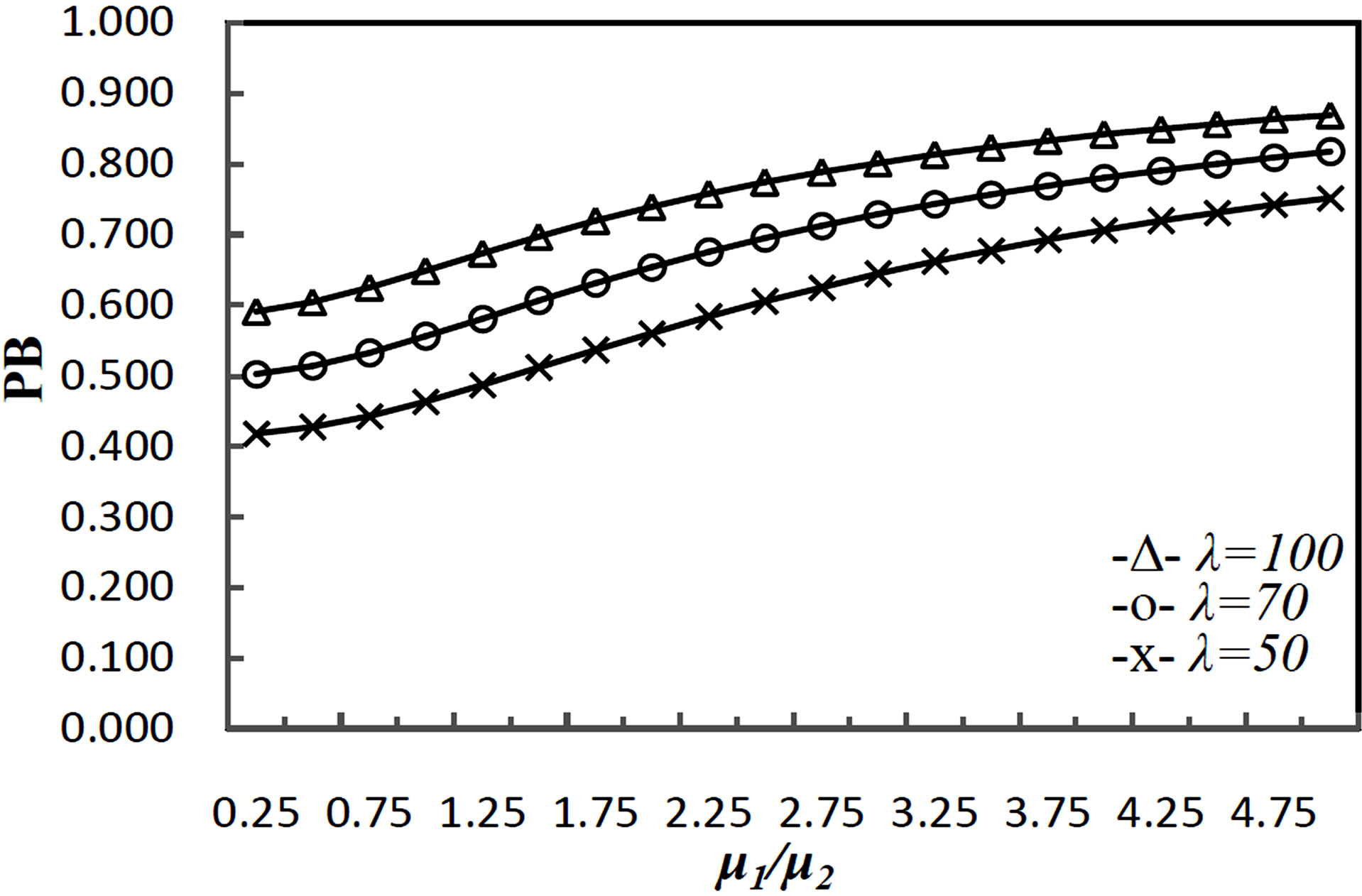
Figure 10. Blocking probability of arrival packets versus μ1/μ2.
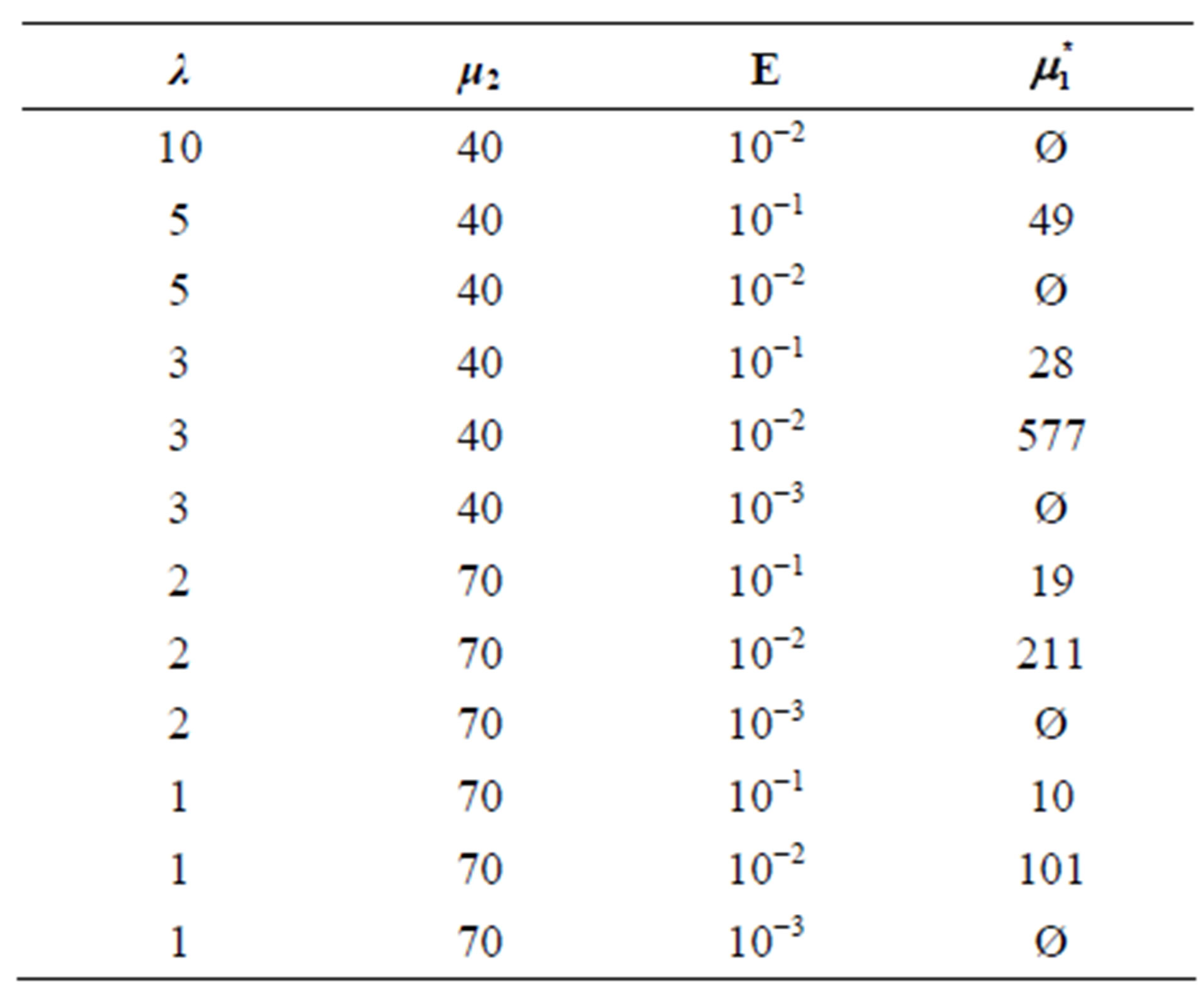
Table 2. Solution results for the problem (19) and (20).
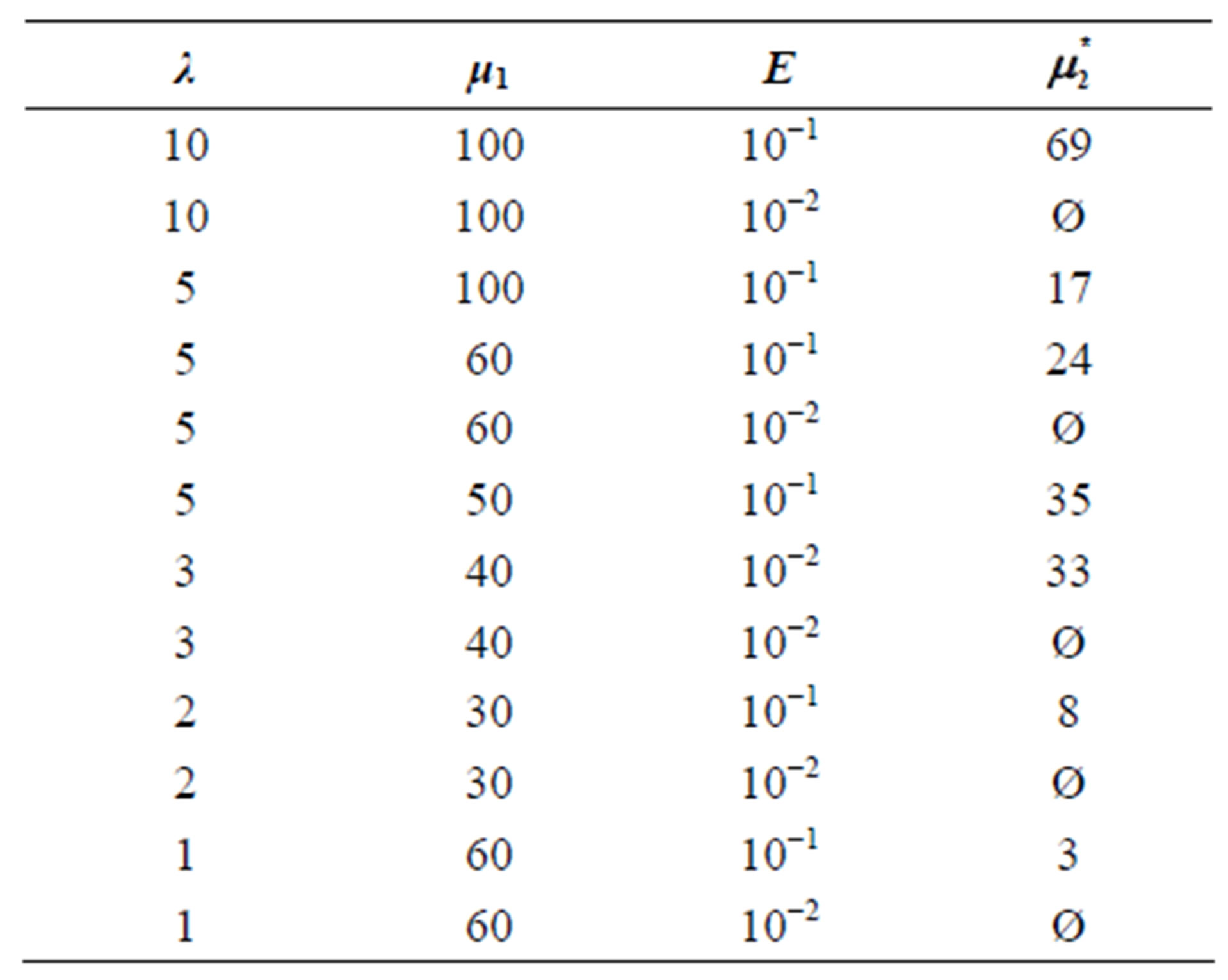
Table 3. Solution results for the problem (21) and (22).
5. Conclusion
As we mentioned above, choosing relevant transceiver and microcontroller components plays important role in assembling sensor devices in sensor nodes, in which data controls should be designed so that packet loss is minimized. Since available QoS metrics based on queuing/buffer management in wired and other wireless networks cannot be applicable in WSNs because of its unique characteristics, new models are required to measure QoS metrics. In this paper the simplest case of queuing/buffering management system-bufferless case were proposed. In order to make trade-off between energy consumption and required hardware specification a quality of services metric—blocking probability were analyzed. Based on the proposed model it gives clear picture on how intensive rates should be chosen in order to reduce data loss. The numerical result of the model gives us the basic research on how determine desirable rate of transmission/receiving and the specification of microcontrollers. Since there are very less researches on this topic, proposed model is satisfactory to determine hardware configuration in terms of transceiver and microcontroller in order to maximize utilization and minimize data loss.
REFERENCES
- I. Akyildiz, W. Su, Y. Sankarasubramaniam and E. Cayirci, “Wireless Sensor Networks: A Survey,” Computer Networks, Vol. 38, No. 4, 2002, pp. 393-422. doi:10.1016/S1389-1286(01)00302-4
- J. F. Kurose and K. W. Ross, “Computer Networking: A Top-Down Approach Featuring the Internet,” 3rd Edition, Addison Wesley, Boston, 2005.
- O. Berder and O. Sentieys, “PowWow: Energy-Efficient HW/SW Techniques for Wireless Sensor Networks,” Proceedings of the Workshop on Ultra-Low Power Sensor Networks, Hannover, 22-25 February 2010, pp. 229- 233.
- M. Escheikh and K. Barkaoui, “Opportunistic MAC Layer Design with Stochastic Petri Nets for Multimedia Ad Hoc Networks,” Concurrency Computation Practice and Experience, Vol. 22, No. 10, 2010, pp. 1308-1324. doi:10.1002/cpe.1581
- A. W. Liehr, K. J. Buchenrieder, “Simulating Inter-Process Communication with Extended Queueing Networks,” Simulation Modelling Practice and Theory, Vol. 18, No. 8, 2010, pp. 1162-1171. doi:10.1016/j.simpat.2009.08.010
- C. Chiasserini and E. Magli, “Energy Consumption and Image Quality in Wireless Video-Surveillance Networks,” Proceedings of 13th IEEE International Symposium on Personal, Indoor and Mobile Radio Communications (PIMRC), Helsinki, 15-18 September 2006, pp. 2357- 2361.
- I. F. Akyildiz, T. Melodia and K. R. Chowdhury, “A Survey on Wireless Multimedia Sensor Networks,” Computer Networks, Vol. 51, No. 14, 2007, pp. 921-960. doi:10.1016/j.comnet.2006.10.002
- T. Qiu, F. Xia, F. Lin, G. Wu and B. Jin, “Queueing Theory-Based Path Delay Analysis of Wireless Sensor Networks,” Advances in Electrical and Computer Engineering, Vol. 11, No. 2, 2011, pp. 3-8. doi:10.4316/aece.2011.02001
- T. Qiu, L. Wang, L. Feng and L. Shu, “A New Modeling Method for Vector Processor Pipeline Using Queueing Network,” 5th International ICST Conference on Communications and Networking, Beijing, 25-27 August 2010, pp. 1-6.
- S. A. Khan and S. A. Arshad, “QoS Provisioning Using Hybrid FSO-RF Based Hierarchical Model for Wireless Multimedia Sensor Networks,” (IJCSIS) International Journal of Computer Science and Information Security, Vol. 4, No. 1-2, 2009, p. 16.
- R. Andriansyah, T. V. Woensel and F. R. Cruz, “Performance Optimization of Open Zero-Buffer Multi-Server Queueing Networks,” Computers and Operations Research, Vol. 37, No. 8, 2010, pp. 1472-1487. doi:10.1016/j.cor.2009.11.004