Journal of Water Resource and Protection
Vol.6 No.10(2014), Article
ID:48190,7
pages
DOI:10.4236/jwarp.2014.610082
Concept of Bed Roughness Boundary Layer and Its Application to Bed Load Transport in Flow with Non-Submerged Vegetation
Ho-Seong Jeon, Makiko Obana, Tetsuro Tsujimoto
Department of Civil Engineering, Nagoya University, Nagoya, Japan
Email: ttsujimoto@genv.nagoya-u.ac.jp
Copyright © 2014 by authors and Scientific Research Publishing Inc.
This work is licensed under the Creative Commons Attribution International License (CC BY).
http://creativecommons.org/licenses/by/4.0/
![]()
![]()

Received 2 May 2014; revised 1 June 2014; accepted 24 June 2014
ABSTRACT
Ecosystem conservation has become one of the purposes in river management as well as flood mitigation and water resources management, and understanding of river flow and morphology in a stream with vegetation becomes important. Recently 2D depth averaged analysis is familiar even in a stream with vegetation by taking account of form drag due to vegetation. However, the shear stress in vegetated area is not properly described because the resistance law due to bed roughness is not reasonably modified in vegetated area. In this study, we discussed the bed roughness boundary layer in flow with non-submerged vegetation to deduce a reasonable relation between U and u* in vegetated area toward improving the analysis of sediment transport. The results show that the modification of resistance law using by thickness, velocity distribution in that layer was found to bring significant improvement of accurate estimation of shear velocity and subsequently the sediment transport. The proposed modification is improved by 2D depth averaged analysis based on this concept, and its application is certificated through flume experiment.
Keywords:Flow with Non-Submerged Vegetation, Boundary Layer, Bed Roughness, Bed Load Transport

1. Introduction
Flood mitigation and ecosystem conservation are simultaneously required in recent river management, and understanding and analysis of flow and river morphology in a stream with vegetation have become important topics in river hydraulics. In particular, river ecosystem is recognized as an interrelating system among flow, sediment transport and morphology and it provides suitable habitat and proper fields for elementary processes of cycling of biophilic elements [1] . Recently, the depth-averaged 2-dimensional model has become familiar with the analysis of river morphology, and the key in this line is how to model riparian vegetation, where vegetation is dealt with as a group of dispersive obstacles to be represented by spatially averaged form drag. The applicability is fine and sometimes it is available to describe the outline of fluvial process there [2] .
In depth averaged model, the resistance law to relate the depth-averaged velocity (U) to the shear velocity (u*) for uniform flow is introduced. If the logarithmic law is applied as velocity profile u(z), Keulegan’s equation obtained by integration the velocity profile along the depth is employed.
 (1)
(1)
where z = vertical distance from the bed; κ = Karman’s constant; h = depth; ks = equivalent sand roughness, Bs(Re*) = function of roughness Reynolds number Re* = u*ks/ν; h = depth; and ν = kinematic viscosity.
In vegetated area, form drag is predominant and velocity profile is uniform (Uv) along the depth only except the thin layer near the bed where the boundary layer is developed to bring a shear flow (see Figure 1), and such a boundary later is considerably thin in general. In Figure 1, the roughness boundary layer thickness is suggested by θv.
The characteristic velocity in vegetated area called Uv is expressed as follows:
 (2)
(2)
where g = gravitational acceleration; Ie = energy gradient of flow, D = diameter; λ = number density of piles; and CD = drag coefficient.
In the conventional depth-averaged analysis for flow with vegetation, the form drag for vegetation is introduced in addition to the bed friction in the vegetated area, but the resistance law due to bed roughness is treated by employing the same equation with that in non-vegetated area (Equation (1)). However, depending on the velocity profile as shown in Figure 1, a proper resistance law should be applied in vegetated area. As mentioned later, though the resistance law is not necessarily sensitive for calculation of depth and depth-averaged flow, it brings underestimation of the shear velocity and subsequently sediment transport rate, and it may not bring a reasonable analysis of sediment transport and subsequent fluvial process.
In this paper, we discuss the bed roughness boundary layer in flow with non-submerged vegetation and deduce a reasonable relation between U and u* in vegetated area to proceed the analysis of sediment transport.
2. Bed Roughness Boundary Layer in Vegetated Area
2.1. Bed Roughness Boundary Layer Thickness in Vegetated Area
Figure 2 shows elaborate measurement of vertical distribution in flow with non-submerged vegetation conducted by Liu et al. [3] , where a group of piles arranged in staggered pattern was utilized as non-submerged vegetation. The thickness of bed roughness boundary layer was found from Figure 2 and the local velocity in the boundary layer was obtained.
The bed roughness boundary layer thickness θv is subjected to the characteristics of vegetation, and dimensional analysis suggests the relation between θv/h and λDh. In Figure 3, the data obtained the measurements by Liu et al. [2] are plotted in Figure 3. By considering that θv may decrease with the vegetation density while it tends to the flow depth with sufficiently disperse density, the following relation is proposed as a favorable formula to estimate the bed roughness boundary layer thickness.
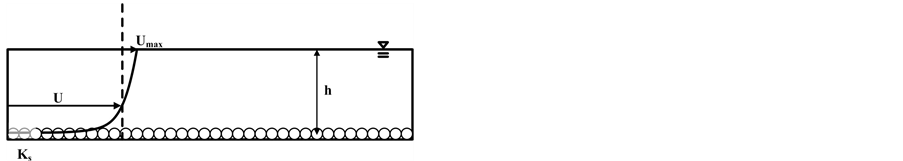
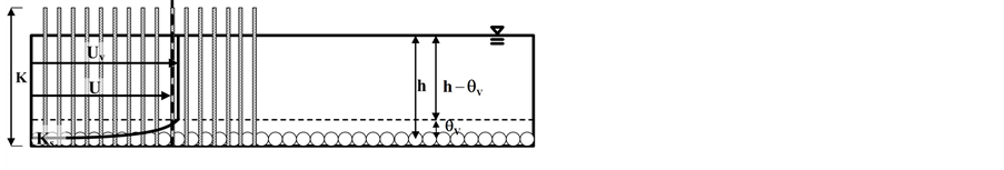
Figure 1. Vertical distribution of velocity in vegetated area.
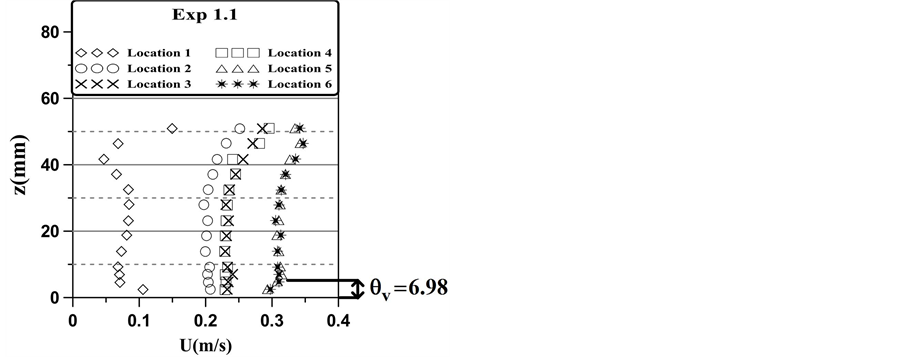
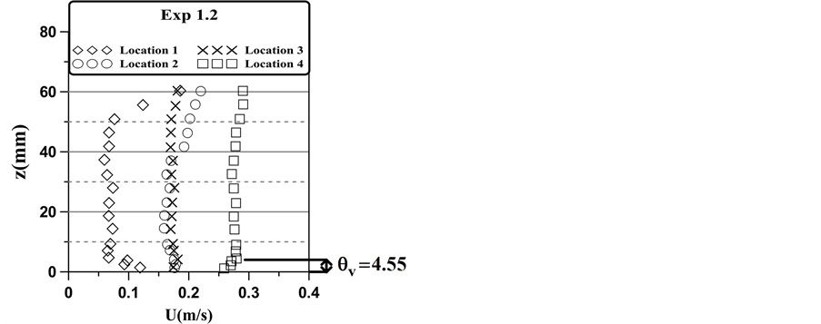
Figure 2. Velocity profile in vegetated area measured by Liu et al.
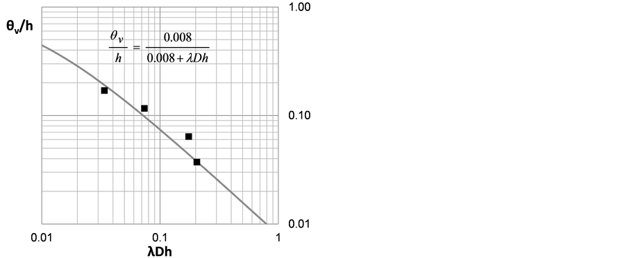
Figure 3. Relation between θv/h and λDh.
 (3)
(3)
2.2. Velocity Distribution in Bed Roughness Boundary Layer in Vegetated Area
Velocity distribution in bed roughness boundary layer in the vegetated area is investigated, and logarithmic law is expected to be applied, which is written as follows.
 (4)
(4)
Though the number of the data is small for each run, the shear velocity in the vegetated area, u*, is evaluated by fitting the logarithmic law for each run, then the data of the all runs are plotted in the defect law expression in Figure 4. Defect law expression is written as follows.
 (5)
(5)
According to this figure, it is recognized that the velocity profile follows the logarithmic law though the number of the measured data for each run is very few.
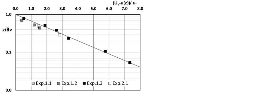
Figure 4. Defect law expression of velocity distribution in bed roughness boundary layer.
2.3. Resistance Law in Vegetated Area
In order to obtain the resistance law to be applied to the vegetated area, velocity distribution is integrated from the bottom to the free surface as follows:
 (6)
(6)
In vegetated area, the shear velocity to govern sediment transport is evaluated by using Equation (6) from the obtained depth-averaged velocity in horizontal 2D flow analysis, and it is applied to evaluate bed load transport rate, entrainment flux of suspended sediment and so on.
3. Flume Experiment and Certification of Model
3.1. Laboratory Experiment
In the laboratory, a model vegetation was prepared by a group of cylinders made of bamboo arranged in staggered pattern (D = 0.25 mm, λ = 0.25/cm2) being set in the interval of 5.0 m in a flume of 20 m long and 0.5 m wide with the constant slope. The bed was rigid.
Firstly, the flow measurements (U and h) were conducted along the centerline of the flume [4] . Then, sand (d = 0.5 cm, σ/ρ = 2.65; d = diameter, σ, ρ = mass density of sand and water) was fed at 1.0 m upstream of the vegetated area with constant volume along the width. The supplied sediment rate was calculated as 0.047 cm2/s. The profile of bed load deposition in the vegetation area was measured along the centerline in the vegetated zone after 12 min. and 20 min. of sediment supply (Figure 5).
3.2. Simulation of depth-Averaged Flow and Comparison with Flume Experiment
The measured data of depth and depth-averaged velocity, U and h, are plotted in Figure 6 to be compared with the results of 2D-depth averaged mode.
The calculation was conducted by using a program developed for horizontal 2D depth-averaged flow where the bed friction and the form drag due to vegetation are taken into account.
 (7)
(7)
 (8)
(8)
 (9)
(9)
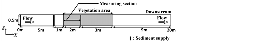
Figure 5. Experimental Flume.
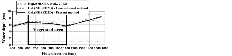
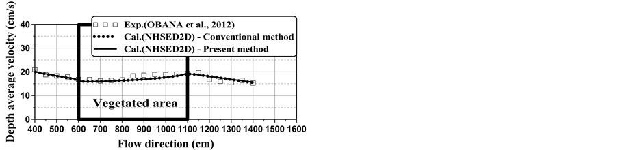
Figure 6. Comparison between measured and calculated results of depth and depth-averaged velocity.
 (10)
(10)
 (11)
(11)
 (12)
(12)
where (x, y) = longitudinal and lateral directions, (U, V) = depth-averaged velocity in x and y direction; zb = bed elevation; (τbx, τby) = bed shear stress in x and y directions; (Dx, Dy) = diffusion terms in x and y directions; νt = kinematic eddy viscosity. (Fx, Fy) = x and y components of form drag due to vegetation; and Cf = friction coefficient defined as (U/u*)2.
In the conventional way, Keulegan’s equation (Equation (1)) is employed for Equation (11) to both non-vegetated and vegetated areas. While, when the present method is applied, Equation (5), which is presently proposed for flow with non-submerged vegetation, is employed for Equation (11) in the vegetated area.
As shown in Figure 6, the depth and the depth-averaged velocity can be well described even by using the conventional way.
As for the shear velocity, which has not directly measured in the experiment, the calculated one by the conventional model may be appreciably underestimated as shown in Figure 7.
3.3. Bed Load Transport and Deposition in Vegetated Area
Bed load transport can be described by the formula proposed by Ashida & Michiue [4] , and written as follows.
 (13)
(13)
where qB, qB* = bed load transport rate and its dimensionless expression;  = Shields number; and τ*c = dimensionless critical tractive force.
If bed load transport formula by Ashida & Michiue [5] is applied to evaluating the equilibrium transport rate, the supplied sediment in the present experiment (0.047 cm2/s) is less than the equilibrium one (0.062 cm2/s) in the non-vegetated area but excessive than the equilibrium one (0.036 cm2/s) in the vegetated zone. Thus, bed load sediment deposits just upstream of the vegetated area and the upstream part of the vegetated area.
In Figure 8, longitudinal profile of bed load deposition with time is depicted with the measured profile in the vegetated area at 12 min. and 20 min after sediment supply. As for the deposition of bed load in the upstream of
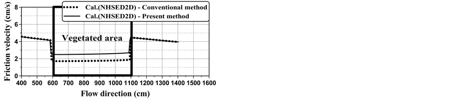
Figure 7. Calculated results on shear velocity.
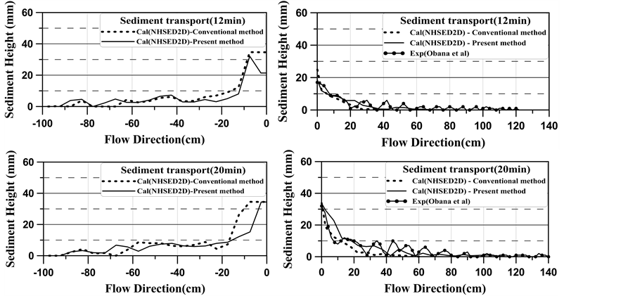
Figure 8. Deposition profile of bed load sediment.
the vegetated zone, we did not conduct the measurement in the flume experiments.
The calculated results, where we employed the conventional resistance law and the presently proposed one for the vegetated area, are compared with the measured data. The present model can describe the deposition profile with the steeper downstream slope with the faster migration because of the higher value of the shear stress, and it shows better conformity with the experimental result compared with the conventional model. Thus, it is concluded that introduction of the present proposal of the resistance law based on the concept of bed roughness boundary layer in vegetated area can bring accurate description of fluvial process in vegetated area.
4. Conclusion
Recently, 2D horizontal depth-averaged flow model becomes familiar to be recognized as powerful means of stream with vegetation by adding the form drag of vegetation. Though it is expected to apply fluvial process of streams with vegetation, the shear stress may be underestimated and fluvial process may not be properly described. In this study, we discussed the bed roughness boundary layer in flow with non-submerged vegetation to deduce a reasonable relation between U and u* in vegetated area toward improving the analysis of sediment transport. The modification of the resistance law by introducing the bed roughness boundary layer brings less change in flow calculation represented by depth and depth-averaged velocity but significant improvement of accurate estimation of shear velocity and subsequently the sediment transport. The proposed modification of the resistance law in the vegetated area will improve accuracy in description of other aspects involved in fluvial processes.
References
- Tsujimoto, T. (2010) Structure and Functions of River Ecosystem—Approach from Ecohydraulics. Proceedings of 10th International Symposium on Ecohydraulics, Invited Lecture, IAHR, Seoul, CD-ROM.
- Tsujimoto, T. (1999) Flow and Fluvial Processes in Streams with Vegetation. Journal of Hydraulic Research, 37, 789-803. http://dx.doi.org/10.1080/00221689909498512
- Liu, D., Diplas, P., Fairbanks, J. and Hodges, C. (2008) An Experimental Study of Flow through Rigid Vegetation, Journal of Geophysical Research, 113, Article ID: F04015.
- Obana, M, Uchida, T. and Tsujimoto, T. (2012) Deposition of Sand and Particulate Organic Matter in Riparian Vegetation. Advances in River Engineering, JSCE, 47-52. (in Japanese)
- Ashida, K. and Michiue, M. (1972) Hydraulic Resistance of Flow in an Alluvia Bed and Bed Load Transport Rate. Proceedings of JSCE, No. 206, 59-69. (in Japanese)