Journal of Water Resource and Protection
Vol.5 No.1(2013), Article ID:26986,11 pages DOI:10.4236/jwarp.2013.51001
Rainfall Prediction Model Improvement by Fuzzy Set Theory
1Department of Civil Engineering, Alabama Agricultural and Mechanical University, Normal, USA
2Department of Computer Science, Alabama Agricultural and Mechanical University, Normal, USA
3College of Agriculture, Food Sciences, and Sustainable Systems, Kentucky State University, Frankfort, USA
4Department of Mathematics, Alabama Agricultural and Mechanical University, Normal, USA
Email: mahbub.hasan@aamu.edu, fshi_xz@yahoo.com, tsegaye.tefery@kysu.edu, nesar.ahmed@aamu.edu, salam.khan@aamu.edu
Received September 19, 2012; revised October 25, 2012; accepted November 4, 2012
Keywords: Fuzzy Sets; Prediction; Rainfall; Water Resources
ABSTRACT
This paper presents the improvement of the fuzzy inference model primarily developed for predicting rainfall with data from United States Department of Agriculture (USDA) Soil Climate Analysis Network (SCAN) Station at the Alabama Agricultural and Mechanical University (AAMU) Campus for the year 2004. The primary model was developed with Fuzzy variables selected based on the degree of association of different factors with various combinations causing rainfall. An increase in wind speed (WS) and a decrease in temperature (TP) when compared between the ith and (i−1)th day were found to have a positive relation with rainfall. Results of the model showed better performance after introducing the threshold values of 1) relative humidity (RH) of the ith day; 2) humidity increase (HI) when compared between the ith and (i−1)th day; and 3) product (P) of increase in wind speed (WS) and decrease in temperature (TP) when compared between the ith and (i−1)th day. In case of the improved model, errors between actual and calculated amount of rainfall (RF) were 1.20%, 2.19%, and 9.60% when using USDA-SCAN data from AAMU campus for years 2003, 2004 and 2005, respectively. The improved model was tested at William A. Thomas Agricultural Research Station (WTARS) and Bragg farm in Alabama to check the applicability of the model. The errors between the actual and calculated amount of rainfall (RF) were 3.20%, 5.90%, and 1.66% using USDA-SCAN data from WATARS for years 2003, 2004, and 2005, respectively. Similarly, errors were 10.37%, 11.69%, and 25.52% when using SCAN data from Bragg farm for years 2004, 2005, and 2006, respectively. The primary model yielded the value of error equals 12.35% using USDASCAN data from AAMU campus for 2004. The present model performance was proven to be better than the primary model.
1. Introduction
Application of fuzzy set theory has rapidly increased with establishing its utility in numerous areas of the scientific world. Any system consisting of vague and ambiguous input variables may contribute to an ultimate effect. In fuzzy logic approach, it is possible to express crisp intervals in terms of linguistic subsets by fuzzy expressions like low, medium, high, good, moderate, poor etc. Each of these expressions represents the sub-range of the entire variability of the variables concerned [1-7]. Weather prediction has been done using conventional probability theory. Here, fuzzy set theory, as an alternate method has recently been applied to develop a model for predicting rainfall as it is concerned with ambiguities and vagueness. The fuzzy logic possibility and its degree of effect due to the ambiguous input variables are considered by some as being generated in the human mind and is often referred to as expert knowledge. This expert knowledge is the accumulation of knowledge and ideas as a result of the expert’s experience in a particular system; hence, decision-making processes may be considered as fuzzy expressions perceived by the expert [8]. Expert knowledge is expressed as a vague or ambiguous expression and not in form of any quantified value. Based on the generated idea that the possibility and degree of effect from vague and ambiguous inputs exists, then the knowledge based rules can be expressed in the form of statements, called fuzzy statements or production rules. These statements consist of antecedent (conditional part) and consequent (inference or effect due to the vague and ambiguous conditional variables) part. In predicting weather condition, there are factors in the antecedent and consequent parts are vague and ambiguous in nature. Their effect is generated in the mind of the expert with more or less accuracy. The decision-makers use their knowledge with logic and then generate algorithms in their mind [9,10].
Application of the concept of fuzzy set theory in soil, crops, water management remain in its infant stages due to the lack of awareness of potential of fuzzy set theory in the field of the above mentioned areas. Weather forecasting is one of the most imperative and demanding operational responsibilities carried out by meteorological services all over the world. It is a complicated procedure that includes numerous specialized fields of knowledge and skill. The task is intricate because in the field of agro-meteorology decisions are heavily intertwined in the visage of uncertainty associated with the weather systems.
The primary fuzzy inference model was developed successfully for predicting rainfall using the antecedent variables of increase in wind speed and decrease in temperature, hereafter termed WS and TP, respectively, when compared between the ith and (i−1)th day. Improvement of the primary model was necessary to enhance its performance in the sense of preciseness and to improve the match between actual and calculated values of rainfall, hereafter termed RF.
2. Fuzzy Systems and Rules
In our everyday life, we encounter numerous problems that do not have any ready answer except making a decision based on our past experiences [1]. These inferred decisions are assessed and validated with actual situations by either observations or measurements.
Fuzzy inference is the actual process of mapping with a given set of input and output through a set of fuzzy rules. Figure 1 shows the general structure of a fuzzy system. Steps for successful application of modeling through a general fuzzy system are as follows:
1) Fuzzification of the input and output variables by considering appropriate linguistic subsets (NL, NS, ZE, PS, and PL the meanings have been described in a tabular form in Figure 2).
2) Construction of appropriate production rules that are comprised of antecedent and consequent parts of IF. Then algorithms with logic based on past experiences of the decision makers.
3) The implication part of a fuzzy system is defined as the shaping of the consequent part based on the premise (antecedent) part and the inputs are fuzzy subsets [1].
4) This is necessary to defuzzify the output results to obtain a crisp value results as these appear as fuzzy subset. Defuzzification is frequently carried out by center of gravity method [8].
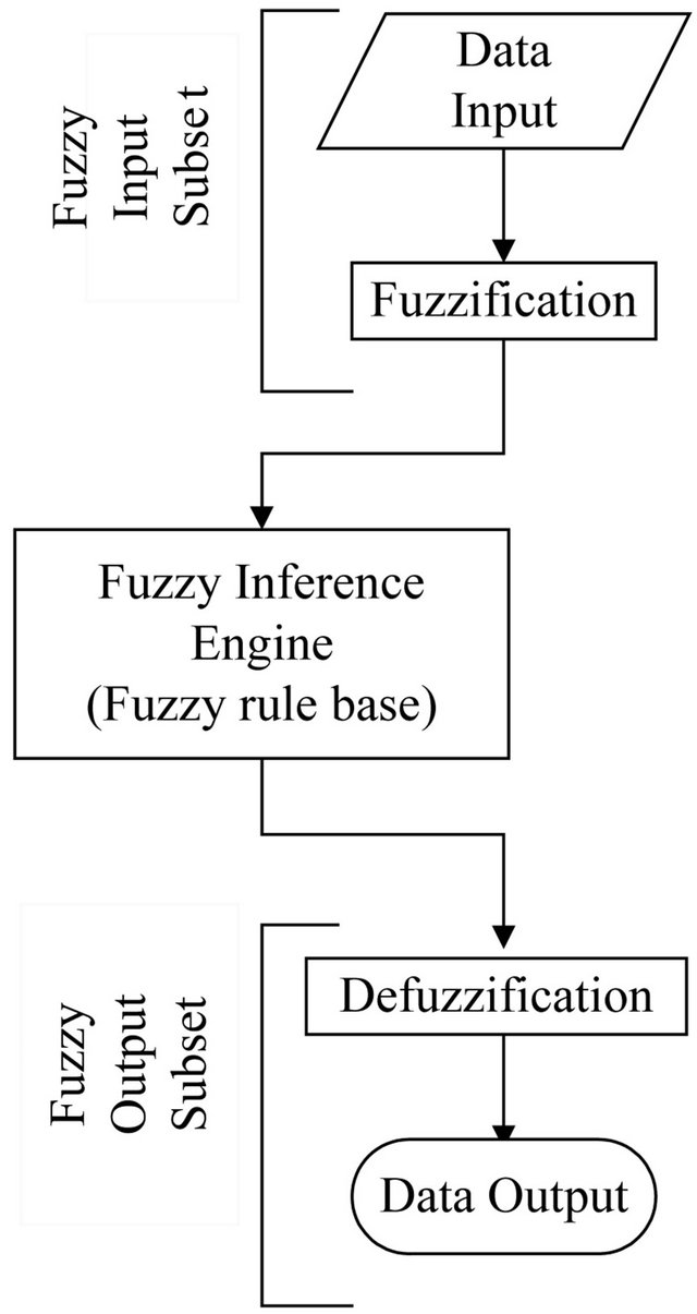
Figure 1. Basic structure of a fuzzy inference model.
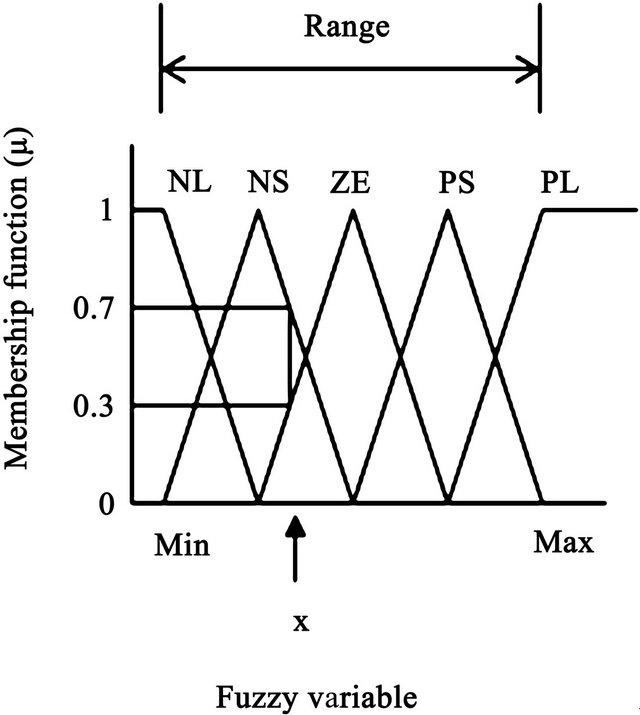
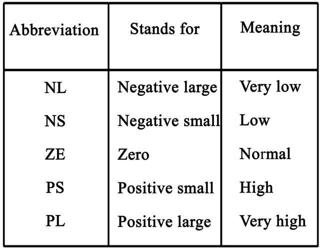
Figure 2. Triangular functional diagram and method for calculating membership function (μ) and corresponding fuzzy levels.
2.1. Fuzzification
Figure 2 shows the mathematical approach to derive the membership functions and fuzzy levels of a fuzzy variable. For example, value of x of a fuzzy variable yields two membership functions (µ1) 0.3 and (µ2) 0.7 and fuzzy levels ZE and NS (point of intersections), respectively. Examples of production rules can be shown as follows:
IF wind speed (WS) is strong and average temperature (TP) is lower THEN rainfall is moderate. (1)
IF wind speed (WS) is strong and average temperature (TP) is moderate THEN rainfall is moderate. (2)
In the calculation procedure, the range between the minimum (Min) and maximum (Max) value of any fuzzy variable is divided into a suitable numerical scale in ascending order starting from the minimum value. Figure 2 shows the range and the fuzzy levels for any fuzzy set of object in a triangular functional diagram. Here, the range has been divided into 5 equal sub-ranges representing ascending ordered fuzzy levels and are abbreviated: NL, NS, ZE, PS, and PL. Abbreviations and meanings for these five fuzzy levels are shown in Figure 2.
2.2. Min-Max Composition
Figure 2 shows that one fuzzy variable x yields two membership functions µ1 = 0.7 and µ2 = 0.3 and their fuzzy levels are NS and ZE, respectively. Hence, if there are two fuzzy variables in antecedent parts as in equation 1 or 2, there will be four membership functions (µ) and four respective fuzzy levels obtained after fuzzification. Refer to Figure 3, membership functions µ1 = 0.2 and µ2 = 0.8 and their fuzzy levels of WS are ZE and PS, respectively and membership functions µ1 = 0.3 and µ2 = 0.7 and respective fuzzy levels of TP are ZE and NS, respectively. These values are considered to form a table to yield the membership functions (µ) and their fuzzy levels for the inference part of production rules. Here, rainfall is shown in Equations (1) and (2).
Fuzzy levels for the production rules are shown in Figure 3 as follows:
IF WS is ZE and TP is NS THEN RF is NS. (3)
IF WS is PS and TP is NS THEN RF is ZE. (4)
IF WS is ZE and TP is ZE THEN RF is ZE. (5)
IF WS is PS and TP is ZE THEN RF is ZE. (6)
Here fuzzy level for RF are (THEN parts) NS, ZE, ZE, and ZE in Equations (3)-(6) are selected based on logic and that should give the lowest percentage of error between calculated and predicted value of rainfall. Now taking the minimum values of the membership functions (µ) for individual equations will yield the values of membership functions as follows:
IF WS is ZE(0.2) and TP is NS(0.7) THEN RF is NS (0.2).
(7)
IF WS is PS(0.8) and TP is NS(0.7) THEN RF is ZE (0.7).
(8)
IF WS is ZE(0.2) and TP is ZE(0.3) THEN RF is ZE (0.2).
(9)
IF WS is PS(0.8) and TP is ZE(0.3) THEN RF is ZE (0.3).
(10)
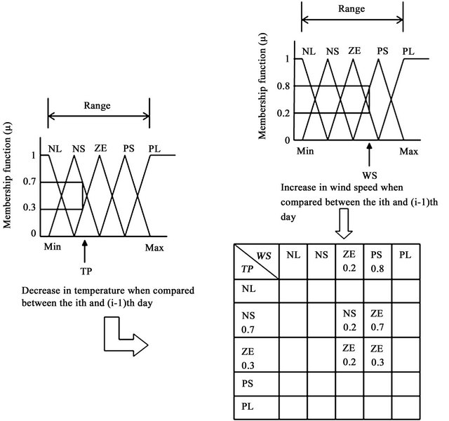
Figure 3. Method for calculating membership function (μ) and corresponding fuzzy levels by min-max composition.
Out of Equations (7)-(10), there is only one NS fuzzy level and three ZE fuzzy levels for RF. Hence, in this kind of situation there NS0.2 is considered without any option. In the remaining Equations (8)-(10), fuzzy levels are the same for rainfall. In this situation, the maximum value of membership function out of ZE(0.7), ZE(0.2), and ZE(0.3) is ZE(0.7). Finally, two fuzzy levels NS and ZE for rainfall and their membership functions NS(0.2) and ZE(0.7) are obtained. This above mathematical calculation procedure is called min-max composition.
2.3. Defuzzification
Membership functions NS(0.2) and ZE(0.7) and their fuzzy levels NS and ZE, respectively are available from the min-max composition and can be plotted in another triangular functional diagram for rainfall where the values of membership functions NS(0.2) and ZE(0.7) and their fuzzy levels NS and ZE are super imposed [8]. A new polygon is formed as shown by thick lines in Figure 4. Now the calculated coordinate (x-axis value) of the center of gravity in this polygon yields RF. This method of determining the predicted value of RF is termed defuzzification.
3. Primary Model
The primary model was developed using data from United States Development of Agriculture (USDA) Soil Climate Analysis Network Station at the Alabama Agricultural and Mechanical University (AAMU) Campus for 2004. Based on the trend of that data, it was observed that in most cases RF was found to occur when a condition of an increase in WS and a decrease in TP when compared between the ith and (i−1)th days exists.
Result of the primary model using data from April 1 to 30 of 2004 from AAMU campus showed that the timing of predicted RF occurrences undisputedly matches with the actual RF (Figure 5). But some discrepancies in matching between the amount of actual and predicted values are yet to be improved. The primary model was developed based on some assumptions on the values of factors as indicated in Figure 6.
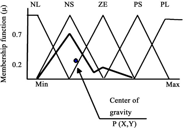
Figure 4. Defuzzification by center of gravity method.
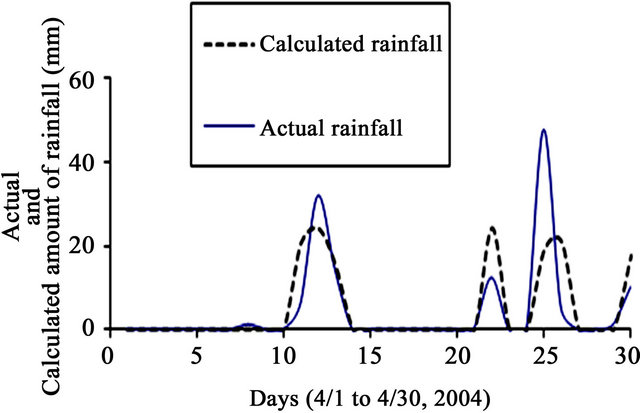
Figure 5. Actual and calculated amount of rainfall (RF) in mm during April 1 to 30, 2004 using AAMU campus data.
Figure 6 further shows 2 boundary values of RH. The lowest bound was denoted by A and the highest value was denoted by B. These two values were different during three seasons of a year. These three seasons are as follows:
1) January 1 to April 31;
2) May 1 to September 30;
3) October 1 to December 31.
Values of RH beyond the highest limit B was considered to cause an immediate RF. Similarly, values of RH less than the value of A was considered to never cause a RF occurrence. Values between A and B were considered to be the possible zone of RF occurrence with the additional consideration of HI value. Region between A and B would cause a RF if the HI value was greater than 10 when compared between the ith and (i−1)th day. But the value of HI ≤ 10 might also contribute to a RF occurrence if the value of P (product of WS and TP) when compared between the ith and (i−1)th day was greater than 4 else there was no possibility of having a RF.
4. Improvement of the Primary Model
This model was developed with careful consideration that the individual result of calculated value of RF should match the actual value of RF. Moreover, an additional consideration was that the calculated amount of RF should not be a value of RF which is more than the actual value of RF with an objective to avoid the misjudgment of falsely predicting a flood (if the calculated value of RF is much higher than actual value of RF) or a misjudgment on minimum available soil moisture in case of moderate or very low value of calculated RF. Hence, the calculated value of RF amount was strongly desired to match with the actual value of RF. Figure 5 further shows a good match of the calculated timing of RF with the actual RF occurrences, but a fairly wide discrepancy between the calculated and actual values of RF. Moreover, it gives an over prediction of RF which is not considered to be on the safe side. Focusing on the real data and the total results, it was further observed that the value of calculated RF does not follow the same trend of decrease or increase with similar range of data of WS and TP when compared between the ith and (i−1)th day, especially when the actual value of RF is in the higher range. Hence, improvement of the primary model to predict a value of RF closer to actual RF was considered an important objective.
The primary model was then carefully examined for possible ways to get a better match between the calculated and actual values of RF. Figure 6 shows the threshold values of the variables and how their ranges were considered in the primary model. Figure 7 represents the improved version of Figure 6 that has been considered in the improved model.
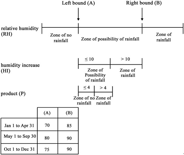
Figure 6. Threshold values of additional factors for predicting rainfall (RF).
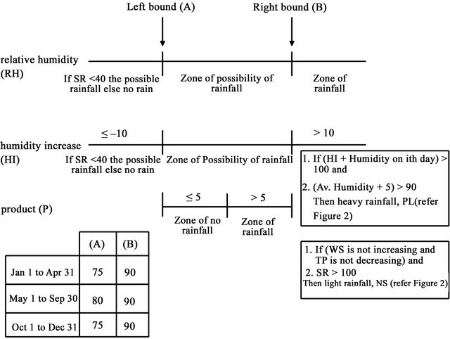
Figure 7. Threshold values and ranges of the factors for predicting RF for the improved model.
Analyzing the initial results and raw data, different assumptions and threshold values were considered on RH on ith day, HI when compared between the ith and (i−1)th day and value of (P) of WS and TP were as follows.
4.1. Threshold Boundaries
Two threshold limits, left bound (A) and right bound (B) were reselected. Values for (A) and (B) were different than in the primary model during January 1 to April 31 as shown in Figures 6 and 7.
4.2. Assumptions on RH
1) If the value of RH on ith day is >(B) then there is a RF occurrence;
2) If the value of RH on ith day is in between (A) and (B) then there is a possibility of RF occurrence; and 3) If the value of RH on ith day is <(A) and value of solar radiation SR is <40 then there is a RF occurrence else there is no RF occurrence.
4.3. Assumptions on HI between (A) and (B)
1) If the HI between the ith and (i−1)th day > 10 and it is beyond (B) then there is a RF occurrence with a fuzzy level of PS only if
a) the sum of HI between the ith and (i−1)th day and Humidity on the ith day > 100 and b) value of (Humidity + 5) > 902) If HI between the ith and (i−1)th day is within the range of ≤10 and >10 then there is possibility of RF occurrence, and 3) If HI between the ith and (i−1)th day is ≤10 and SR is <40 then there is a possibility of RF occurrence else there will be no RF occurrence.
4.4. Assumptions on P between the Range of Threshold Values (A) and (B)
1) If the value of P of WS and TP is ≤5 then there is no RF occurrence2) If the product of WS and TP is >5 then there is no RF occurrence only if a) WS is not increasing and TP is not decreasing and b) SR > 100 then there will be a light RF occurrence with fuzzy level NL.
Actual data showed that most of the time, there is a possibility of RF occurrence when there is a trend of decreasing the value of SR comparing the previous 1 or 2 days. Hence, to improve the primary model a preliminary min-max composition was done by fuzzifying WS and TP to yield ø, representing the condition that is favorable for a RF occurrence. Membership functions (µ) and their corresponding fuzzy levels obtained from preliminary min-max composition were again considered along with the membership functions (µ) and their corresponding fuzzy levels of SR to do the secondary min-max composition finally to yield the predicted RF. The above case was considered only if the value of SR has a decreasing trend for two previous consecutive days. Otherwise no need of fuzzification of SR was considered where the preliminary min-max composition was done to yield the predicted value of RF. Figure 8 represents the model structure with secondary min-max composition when the value of solar radiation has a decreasing nature for two consecutive days else predicted value of RF was calculated by defuzzification right after the preliminary minmax composition operation.
4.5. Percentage of Error Calculation
Percentage of error and the improved model performance was evaluated by the following equation:
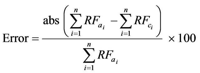 (11)
(11)
Here,  is the actual amount of rainfall in mm,
  is the calculated amount of rainfall in mm. “n” is total number of data.
5. Results and Discussions
5.1. Selection of Variables in the Primary Model
Fuzzy variables of increase in wind speed (WS) and decrease of temperature (TP) between the ith and (i−1)th day were a good choice in developing the model for predicting RF in the primary model. In reality, fuzzy inference models are involved with the variables which are perceived by the experts who are responsible for inferring the consequence part of the production rule. That means a fuzzy inference model reflects the scenario of thinking and decision-making process by an expert knowledge. The primary model also described a secondary method how the variables can be selected without even being perceived by an expert. The fuzzy variables were chosen by judging the degree of involvement or association of the variables of WS and TP between the ith and (i−1)th day against occurrence of RF. Hence, the variables WS and TP between the ith and (i−1)th day were used in this model.
5.2. Selection of Fuzzy Levels for the Inference Part of Production Rule Table in the Primary Model
Selection of the fuzzy levels in the inference portion of the production rules is a cumbersome process by trial and error method. There are 5 (NL to PL) × 5 (NL to PL) = 25 fuzzy variables for the inference part shown inside the Table of Figure 3. Number of fuzzy levels is doubled if it needs the secondary min-max composition as explained in Figure 8. The most logical approach for the fuzzy variables for RF was followed in the computer program, selecting the one that yielded the lowest percentage of error using Equation (11). Depending on the scenario of the system, fuzzy levels in the inference part of the production rule must have either an ascending or descending nature, from NL to PL or PL to NL. It requires a skillful and logical approach to determine the fuzzy variables for the consequent part with respect to the fuzzy variables in the antecedent part of production rule. The value for lowest percentage of error of the primary model was 12.35 using Equation (11).
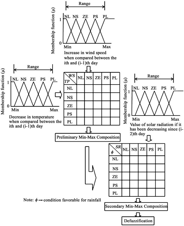
Figure 8. Concept of considering solar radiation (SR) in the improved model.
5.3. Maximum Amount of RF
Real data for RF showed that AAMU campus weather station had only 5 actual RF events exceeding 50 mm in 2004. The maximum RF was 93 mm which is rare for AAMU campus location. Considering Figure 4, if RF data more than 50 mm is considered, the region of maximum RF (around PL) will be in a sparsely populated data region for RF having more than 50 mm, when compared with the RF data that falls within the regions of NL, NS, ZE, and PS. Regions from NL to PS will have more densely populated data while compared to regions from PS to PL with cases more than 50 mm actual RF for 5 times occurrences only in 2004. Hence, in the improved model, total range (refer to Figure 2 or 3) was divided into 4 sub-ranges to make a uniform distribution of RF data among fuzzy levels from NL to PL, the total range (refer to Figure 4) was divided into 4 sub-ranges to represent the following:
1) first sub-range between NL and NS was taken equal to total range divided by 8 (50 ÷ 8 = 6.25);
2) second sub-range between NS to ZE was taken equal to total range divided by 4 (50 ÷ 4 = 12.50);
3) third sub-range between ZE to PS was taken equal to total range divided by 2 (50 ÷ 2 = 25.00); and 4) fourth sub-range between ZE to PS was taken equal to total range divided by 1 (50 ÷ 1 = 50.00).
Therefore, the sub-ranges were (0 to 6.25), (6.25 to 12.50), (12.50 to 25.00), and (25.00 to 50.00) mm.
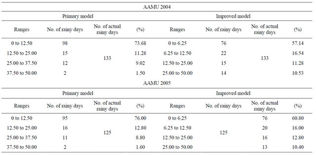
This means, widening the bases of triangles in Figure 4 intersect with the x-axis at 0, 6.25, 12.50, 37.50, and 50.00. In case of the primary model values of the subranges were (0 to 12.50), (12.50 to 25.00), (25.00 to 37.50), and (37.50 to 50.00), respectively. The primary model was developed with equal intervals of the triangular fuzzy levels where as the sub-ranges in the improved model were considered with multiplicative factors of the total range. The improved model further excluded zero RF. Hence, number of zero RF days was discarded in the calculation procedure. Figure 9 shows the predicted and actual values of RF during April 1 to 30, 2004. Table 1 shows the differences in data distribution among the subranges between the primary model and the improved model when AAMU data were used for the years of 2004 and 2005. As the actual RF exceeded 50 mm only for 5 times occurrences, very few compared with the total number of actual RF occurrences, and were considered to be beyond PL. Hence, considering the value of maximum RF as 50 mm was justifiable.
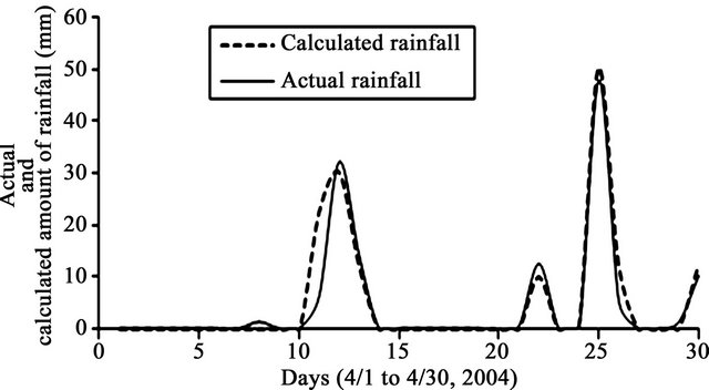
Figure 9. Actual and calculated amount of rainfall RF in mm 2004 after primary model improvement during April 1 to 30 using USDA scan data from AAMU campus data.
Table 1. Comparison of the distribution of data caused by two different sub-range selections for the primary and improved models using USDA scan data from Alabama A & M University (AAMU) Campus for years 2004 and 2005.
5.4. Selection of Other Variables and Threshold Values
Based on the fundamental logic of this research that values of WS and TP between the ith and (i-1)th day may result in RF, their fuzzy levels, production rules, ranges of the variables, showed dependency on three other possible factors to match with the actual situation. They need to be considered with their threshold values for matching with the actual and calculated amount of RF. These factors are 1) RH, 2) HI between the ith and (i−1)th day, and 3) P. Figure 7 represents two boundary values of (A) and (B) for RH. The zone between (A) and (B) is the range for a possible RF and the zone beyond (B) is the zone for RF regardless of any other consideration. Whereas RH less than (A) is the zone for no RF, except when the value of SR is <40, in which SR has been used to improve the primary model performance. The same condition of SR is <40 was considered as contributing to RF occurrence for values of HI ≤ 10 when compared between the ith and (i−1)th day. The range between the values of HI < 10 and >10 may contribute to a RF occurrence. Values of HI > 10 will further depend on two other conditions to cause a RF occurrence but with a fuzzy level of PS. The conditions are as follows:
1) if (HI between the ith and (i−1)th day + Humidity on ith day) > 100, and 2) if (RH on ith day + 5) > 90 then there will be a RF occurrence.
Within the range of possibility of RF occurrence (when the values of HI between the ith and (i−1)th day is within the range <10 and >10), another variable of P (product of values of the variables of WS and TP when both factors were compared between the ith and (i−1)th day) was further separated into two ranges. They were as follows:
1) if the value of P is <5 then there will be no RF, and 2) if the value of P is >5 then there will be a RF occurrence but with fuzzy level of NL.
The model illustrated a good agreement between the actual and calculated amount of RF using USDA-SCAN data from AAMU campus for total year of 2004. It should be mentioned that Figure 9 shows the results of the same graph for a period of April 1 to 30, 2004. This graph depicts a good agreement between the calculated and actual amount of RF and their times of occurrence. There were some cases when the actual RF were more than 50 mm. Considering these cases as unusual RF amounts at AAMU campus and its vicinity when compared with several other years, such amount of highest RF was truncated to 50 mm for a single day. Moreover, if this appears to be discriminatory there will be an opportunity for compensation when the final step of this research is completed on the development of the model to represent the amount of RF on an area basis and not a single point basis as it is measured at the weather station by rain gage.
The improved model was tested using the USDA-SCAN stations data of AAMU campus, Bragg and Winfred A. Thomas Agricultural Research Station (WATARS) for different years. Table 2 shows the result of the improved model for WATARS. Value for amount of maximum RF was taken as 50 mm, as it was a reasonable figure for this location. Error for 2003, 2004, and 2005 were 3.20%, 5.90%, and 1.66%, respectively.
From the real data, it was observed that data from January 1 to February 7 in 2002 were missing. Total number of days for was 327 instead of 365. Hence, data for 2002 were not considered for testing the improved model. That would have caused a bit higher value of error as there is the involvement of “n”, means number of data in Equation (11).
Table 3 shows the test results of Bragg location for years 2004 to 2006. In 2003, data from January 1 to August 26 and December 1 were unavailable. Lack of data and reliability of data were there for 2006 that gave the highest value of percentage of error.
Table 2. Results of the improved model using USDA scan data from WTARS.
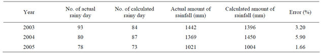
Table 3. Results of the improved model using USDA scan data from Bragg farm.
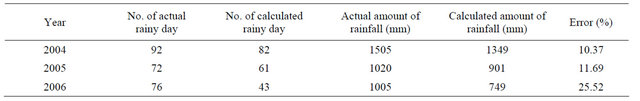
Table 4. Results of the improved model using USDA data from AAMU campus.
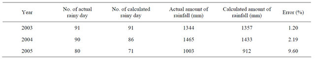
Table 4 represents the results for AAMU location for 2003 to 2005. Here also data for the whole year were unavailable for 2002. Hence, testing the model by using data for 2002 was not performed.
6. Conclusions
Selection of variables and the fundamental logic that the values of WS and TP between the ith and (i−1)th day was a successful attempt to determine the amount of RF and its time of occurrence as the consequent part of the fuzzy inference model. Introducing the idea of threshold values of a) RH of the ith day; b) HI when compared between the ith and (i−1)th day; and c) P was an intellect attempt for the primary model and other additional considerations in the improved model matched well between the actual and predicted amount of RF and also decreased the value of error by using Equation (11). The additional considerations were as follows:
Introducing SR value of <40 and its effect below the left boundary value of RH:
1) introducing of SR value of <40 and its effect below the left boundary value of HI (≤−10);
2) introducing of idea “if (HI + RH of the ith day) > 100 and (RH + 5) > 90” then there will be RF of fuzzy level PS;
3) introducing the idea that “if (wind speed is not increasing or temperature is not decreasing) and SR > 100” then there will be RF with fuzzy level NL;
4) introducing the idea of primary and secondary minmax compositions approach for the condition that SR has a decreasing trend for 2 consecutive days was a successful attempt. Fuzzy levels and membership functions obtained after min-max composition of inference part of the primary model (fuzzifications done for WS and TP were considered as they represent the environmental condition to enhance a RF occurrence when SR value have a decreasing trend for 2 consecutive days. Values of fuzzy levels and membership functions were considered the values for one of the antecedent part of the production rule table and represented as “ ” in Figure 8 for doing the secondary min-max composition where the other variable is SR. The above consideration was taken into account only when the SR value has a decreasing trend for 2 consecutive days else following the same procedure as in the primary model. Values of fuzzy levels and membership functions inside the production rule table were again considered for doing min-max composition with fuzzy levels and membership functions after fuzzification of SR was a successful attempt for improvement of the primary model. Here the membership functions and fuzzy levels after min-max composition for consequent part of the primary model were considered as a conditional step that enhanced the condition for RF occurrence with the decreasing trend of SR for 2 consecutive days.
The above mentioned points include the values of the left (A) and right boundary (B), which are different than the primary model which in turn yields better result for the improved model when compared to the result of the primary model.
7. Acknowledgements
The authors appreciate the Faculty and Staff in the Department of Mechanical and Civil Engineering of Alabama Agricultural and Mechanical University (AAMU) for their constructive suggestions and support. Thanks to Dr. Chance M. Glenn, Sr., Dean of College of Engineering, Technology, and Physical Sciences of AAMU for constant encouragement, Prof. Mohamed Seif, Chairman, Department of Mechanical and Civil Engineering, Alabama A&M University for his institutional and moral support. Prof. Rao Mentreddy and Mr. Daryl Lawson of Alabama Agricultural and Mechanical University are duly acknowledged for reviewing this manuscript. The authors appreciate the cooperation and financial support to the United States Department of Agriculture (USDA) and Natural Resources Conservation Service (NRCS) for conducting this research. The authors also acknowledge the late Robert Metzl for providing data related to this research.
REFERENCES
- Z. Sen and A. Altunkaynak, “Fuzzy System Modeling of Drinking Water Consumption Prediction,” Expert Systems with Applications, Vol. 36, No. 8, 2009, pp. 10801-11400. doi:10.1016/j.eswa.2009.05.025
- A. Altunkaynak, M. Özger and M. Cakmakci, “Water Consumption Prediction of Istanbul City by Using Fuzzy Logic Approach,” Water Resources Management, Vol. 19, No. 5, 2005, pp. 641-654. doi:10.1007/s11269-005-7371-1
- J. Kiska, M. Gupla and P. Nikiforuk, “Energetic Stability of Fuzzy Dynamic Systems,” IEEE Transactions on System, Men and Cybernetics, Vol. 15, No. 6, 1985, pp. 783- 792. doi:10.1109/TSMC.1985.6313463
- E. H. Mamdani, “Application of the Fuzzy Logic to Approximate Reasoning Using Linguistic Synthesis,” IEEE Transactions and Computers, Vol. C-26, No. 12, 1977, pp. 1182-1191. doi:10.1109/TC.1977.1674779
- J. T. Ross, “Fuzzy Logic with Engineering Applications,” McGraw-Hill Inc., New York, 1995.
- Z. Sen and A. Altunkaynak, “Fuzzy Awakening in Rainfall-Runoff Modeling,” Nordic Hydrology, Vol. 35, No. 1, 2004, pp. 31-43.
- L. A. Zadeh, “Fuzzy Sets,” Information and Control, Vol. 8, No. 3, 1965, pp. 338-352. doi:10.1016/S0019-9958(65)90241-X
- M. Hasan, T. Tsegaye, X. Shi, G. Schaefer and G. Taylor, “Model for Predicting Rainfall by Fuzzy Set Theory Using USDA-SCAN Data,” Agricultural Water Management, Vol. 95, No. 12, 2008, pp. 1350-1360. doi:10.1016/j.agwat.2008.07.015
- M. Hasan, M. Mizutani, A. Goto and H. Matsui, “A Model for Determination of Intake Flow Size: Development of Optimum Operational Method for Irrigation Using Fuzzy Set Theory (1),” System Nogaku: Journal of Japan Agricultural System Society, Vol. 11, No. 1, 1995, pp. 1-13.
- T. Hasan and S. Zenkai, “A New Modeling Approach for Predicting the Maximum Daily Temperature from a Time Series,” Turkish Journal of Engineering and Environmental Science, Vol. 23, No. 3, 1999, pp. 173-180.