Journal of Water Resource and Protection
Vol. 3 No. 8 (2011) , Article ID: 6991 , 21 pages DOI:10.4236/jwarp.2011.38066
Geostatistical Modeling of Uncertainty for the Risk Analysis of a Contaminated Site
CGT Center for GeoTechnologies, University of Siena, Arezzo, Italy
E-mail: guastaldi@unisi.it
Received June 12, 2011; revised July 12, 2011; accepted August 14, 2011
Keywords: Uncertainty Modeling, Multivariate Geostatistical Simulations, Risk Analysis, Environmental Pollution, Remediation Project
ABSTRACT
This work is a study of multivariate simulations of pollutants to assess the sampling uncertainty for the risk analysis of a contaminated site. The study started from data collected for a remediation project of a steelworks in northern Italy. The soil samples were taken from boreholes excavated a few years ago and analyzed by a chemical laboratory. The data set comprises concentrations of several pollutants, from which a subset of ten organic and inorganic compounds were selected. The first part of study is a univariate and bivariate statistical analysis of the data. All data were spatially analyzed and transformed to the Gaussian space so as to reduce the effects of extreme high values due to contaminant hot spots and the requirements of Gaussian simulation procedures. The variography analysis quantified spatial correlation and cross-correlations, which led to a hypothesized linear model of coregionalization for all variables. Geostatistical simulation methods were applied to assess the uncertainty. Two types of simulations were performed: correlation correction of univariate sequential Gaussian simulations (SGS), and sequential Gaussian co-simulations (SGCOS). The outputs from the correlation correction simulations and SGCOS were analyzed and grade-tonnage curves were produced to assess basic environmental risk.
1. Introduction
The assessment of the risks associated with contamination by elevated levels of pollutants is a major issue in most parts of the world. Risk is generally taken to mean the probability of the occurrence of an adverse event, in this case contamination above legally and/or socially acceptable levels. Risk arises from the presence of a pollutant and from the uncertainty associated with estimateing its concentration, extent and trajectory. The uncertainty arises from the difficulty of measuring the pollutant concentration accurately at any given location and the impossibility of measuring it at all study. Estimations tend to give smoothed versions of reality (i.e. estimates are less variable than real values) with the smoothing effect being inversely proportional to the amount of data (i.e. directly proportional to the uncertainty). If risk is a measure of the probability of pollutant concentrations exceeding specified thresholds then variability, or variance, is the key characteristic in risk assessment and risk analysis. For this reason, geostatistical simulation provides an appropriate way of quantifying risk by simulateing possible “realities” and determining how many of these realities exceed the contamination thresholds [1].
Since the publication of the first applications of geostatistics to soil data in the early 1980s ([2-6]), geostatistical methods have become popular in soil science, as illustrated by the increasing number of studies reported in the literature.
Geostatistics involves the analysis and prediction of spatial or temporal phenomena, such as metal grades, porosities, pollutant concentrations, price of oil in time, and so forth. Nowadays, geostatistics is simply a name associated with a class of techniques utilized to analyze and predict values of a variable distributed in space or time. Such values are implicitly assumed to be spatially or/ and temporally correlated with each other, and the study of such a correlation is usually called a “structural analysis” or “variogram modeling”. Following structural analysis, predictions at unsampled locations are made using any of the various forms of “kriging” or they can be simulated using “conditional simulations”.
The main geostatistical tools are used to model the local uncertainty of environmental attributes (e.g. pollutant concentrations), which prevail at any unsampled site, in particular by means of stochastic simulation. These models of uncertainty can be used in decision-making processes such as delineation of areas targeted for remediation or design of sampling schemes.
Methods of uncertainty propagation ([7,8]), such as Monte-Carlo simulation analysis, sequential Gaussian simulation and sequential indicator simulation are critical for estimating uncertainties associated with spatiallybased policies in environmental problems and in dealing effectively with risks [9].
The study area was of a contaminated site in northern Italy, previously occupied by a steelworks. This work is based on a data set belonging exclusively to Studio Geotecnico Italiano S.r.l. (Milan, Italy), which has withheld permission to publish the exact geographical location of the site, but this is irrelevant to the purposes of this study. Therefore, the steelworks factory’s site is just roughly located in northwestern Italy in Figure 1, the study area is intentionally enormous compared to the actual site’s area, and the real location is somewhere inside the circle. Moreover, conventional geographical directions are used only in the sections covering descriptions of geomorphology and geology. In the quantitative work reported here easting, northing and depth co-ordinates are given in local units keeping the scale ratio, to protect the confidentiality of the site. In addition, the actual co-ordinate system has been rotated by approximately 90˚ to provide a more convenient data layout. These assumptions, of course, do not affect any results.
The author has conducted a geostatistical study, based on the preliminary reclamation study, to assess the contamination risk associated with the most important heavy metals and hydrocarbons measured at the site. The preliminary reclamation study outlines the reclamation proposed to mitigate the contamination risk based on groundwater analysis. The study here reported is based on soil samples taken from the surface down to different depths up to 20 m and provides a risk analysis method that could be extended to other variables together with results that could form part of a future, definitive reclamation project. The significant number of variables provides the basis for an extensive multivariate study. However, multivariate analysis has been restricted to the subset of these variables with concentration values higher than limits imposed by law.
A univariate geostatistical simulation of several variables is performed independently for each variable and any spatial cross-correlation among the variables is ignored. However, in environmental applications it is common to find pollutants positively or negatively correlated, as is the case with the site used for this project. One way of taking account of this correlation and improving the simulation results is by introducing a correlation correction between pairs of the independently simulated variables [10], another way is utilizing multivariate simulations. Finally, following the validation analysis, the corrected variables were analyzed and compared with those of the co-simulation technique.
The main objective of this study is to assess the uncertainty of the spatial variability of contamination by heavy metals and heavy hydrocarbons in order to perform a risk analysis suitable for the definitive reclamation project.
2. Outlines of Geology and Hydrogeology
The study area is located in the western part of the Po river basin. The quaternary geological cover lies directly over the Tertiary bedrock by means of an erosional contact, the surface of which slopes gently toward northwest. In the study area, however, the sand-silt Pleistocene deposits lie between the quaternary deposits and the Tertiary bedrock [11].
Essentially, the quaternary sediments constituting the shallow quaternary geology of the plain are composed (from the bottom), by heterometric gravel deposits in a sand matrix laid down in the Middle Pleistocene by tributary streams of the Po (fluvial “Riass” period), and gravel fluvial deposits more recent than the present alluvial sediments. In particular, a sub-division can be made on the basis of groundwater reservoirs, which are very well known in this zone [12].
The stratigraphic logs of this area show: 1) a Superficial Complex, with fluvial alluvial and glacial deposits principally composed of coarse gravels characterized by a high permeability thickness of 10 - 30 m (Middle Pleistocene), housing an unconfined aquifer, directly connected to the superficial stream network. Its potentiality is proportional to the thickness of the saturation zone and it is, therefore, highly variable; 2) a very low permeability complex comprising silt-clay sediments lays down in the fluvial environment of the Upper Pliocene-Lower Pleistocene; 3) a Pliocene Complex comprising a series of fairly permeable sand, sometimes with silt-clay intercalations, laid down in a marine environment; 4) a succession of silt, silt-clay and clay levels starting from at least 300 m below the surface [13].
An accurate stratigraphic reconstruction of the study area from the surface to the depth of interest was produced, by analyzing the results of field surveys conducted in the summer 2000 and borehole data collected in the summer 2002. In the earlier survey, the piezometers showed that the geological structure of the area was heterogeneous, with a succession of layers of different and non-constant thicknesses. The more recent survey confirmed the initial geological model. Vertical geological cross-sections were produced and utilized as the geological context for the geostatistical analysis. They show the studied volume completely lays in the above mentioned Superficial Complex.
These cross-sections, combined with the geotechnical laboratory analyses, support the conceptualization of geological model of the study area (Figure 1), characterized as follows starting form the surface (Table 1): Unit 0, mainly constituted by organic terrain (OS) and backfill material (BF), with a significantly variable thickness ranging from centimeters to meters; Unit 1, essentially composed by a unique gravel layer 10 m thick (GS), with a light silty sand fraction (SS), at times with polygenic pebbles with a maximum diameter of 15 cm (PG), and an average hydraulic conductivity of 4.85E-03 cm/s, so with a moderately high permeability in comparison with the other units; Unit 2, polygenic pebbles (PG) and gravel with silty sand (SS) in succession with levels of polygenic gravel and pebbles in an abundant silty-sandy matrix (SG), with a maximum thickness of 10 m, an average hydraulic conductivity of 8.14E-03 cm/s; Unit 3, constituted by sandy silt (SS) moderately coherent, represents the base layer of the aquifer, its bed was not detected, because the borehole stops 24 m below the surface, however granulometric analysis shows an equal percentage of sand, silt and clay, an Atterberg’s liquidity limit less than 30%. These data allow the material to be classified as falling in a range between inorganic silt with low compressibility and inorganic clay with low plasticity. The Lefranc Permeability Tests performed on samples of Unit 3 provided an average hydraulic conductiveity coefficient equal to 0.027E-03 cm/s, denoting a low permeability grade.
3. Method
3.1. Exploratory Raw Data Analysis
There have been two sampling surveys since the recla-
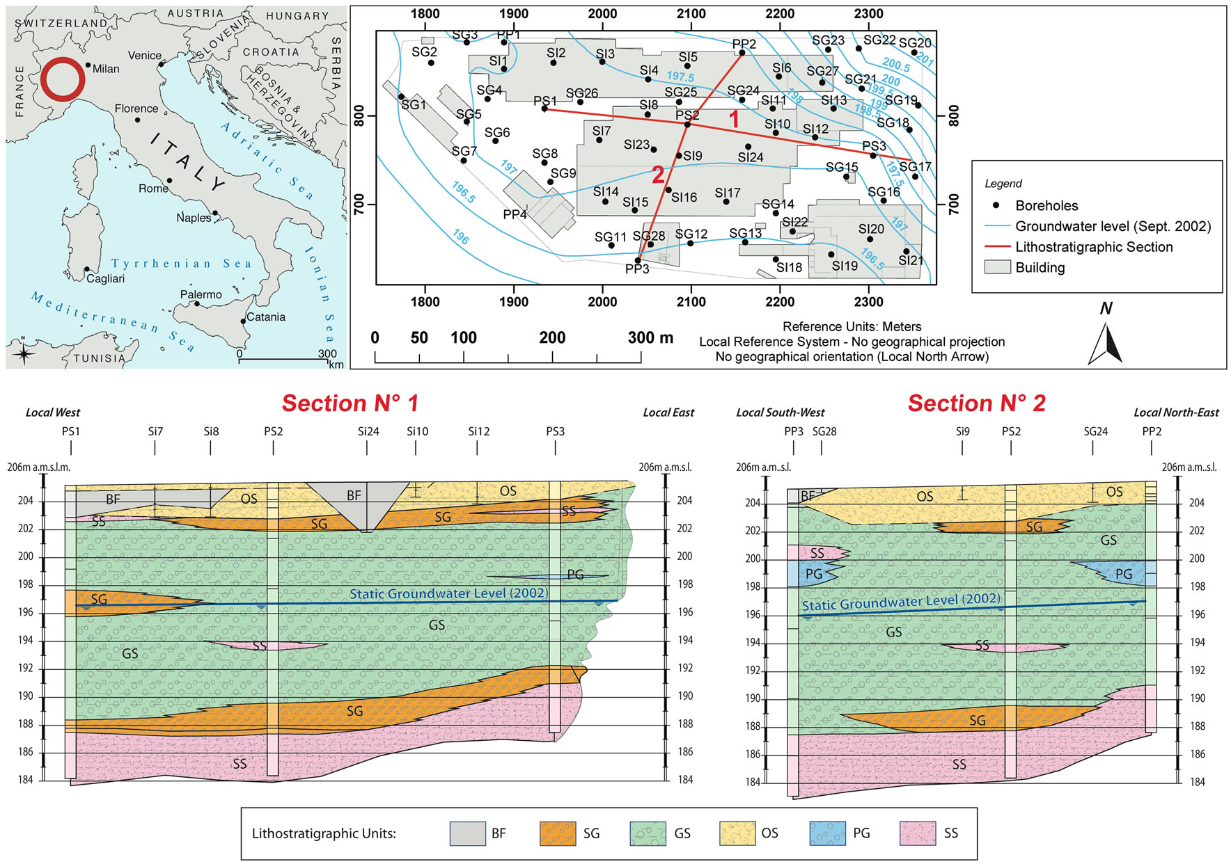
Figure 1. Study area, boreholes, and an example of two lithostratigraphic cross-sections performed (units: BF, Backfilling material mainly constituted by foundry scum; OS, Organic soil and/or backfilling material constituted mainly by sand with pebbles, bricks, rubble, concrete fragments; SG, Sandy gravel; GS, Gravely sand with sparse silt levels; PG, Pebbly gravel; SS, Sandy silt).
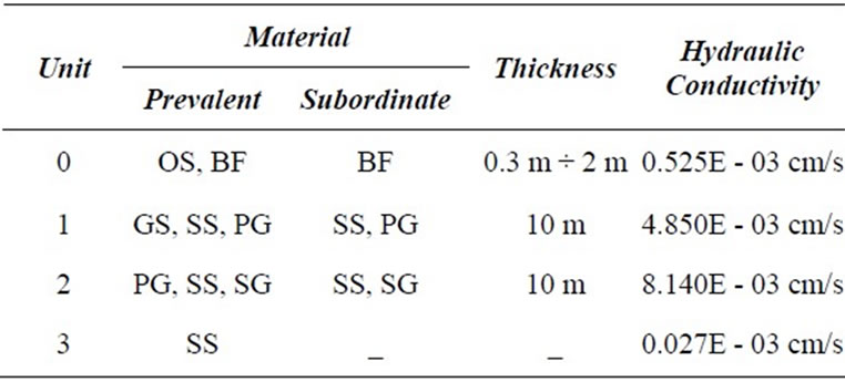
Table 1. Composition and hydraulic conductivity coefficient of principal lithostratigraphic units.
mation project started in 2000. The first took place in the summer of 2000, and comprised five vertical boreholes of 20 m length, which were used as piezometers. Water table measurements were made and ground water analyses were done. The second survey was done between 17 June 2002 and 5 August 2002 and comprised 59 vertical boreholes (percussion type boreholes, continuous type boreholes, deep piezometers, superficial piezometers), together with three surface samples and two samples taken from the bottoms of the wells. The area measured by 276 samples, covers almost the entire zone occupied by the former industrial complex, within an area of 600 m × 250 m.
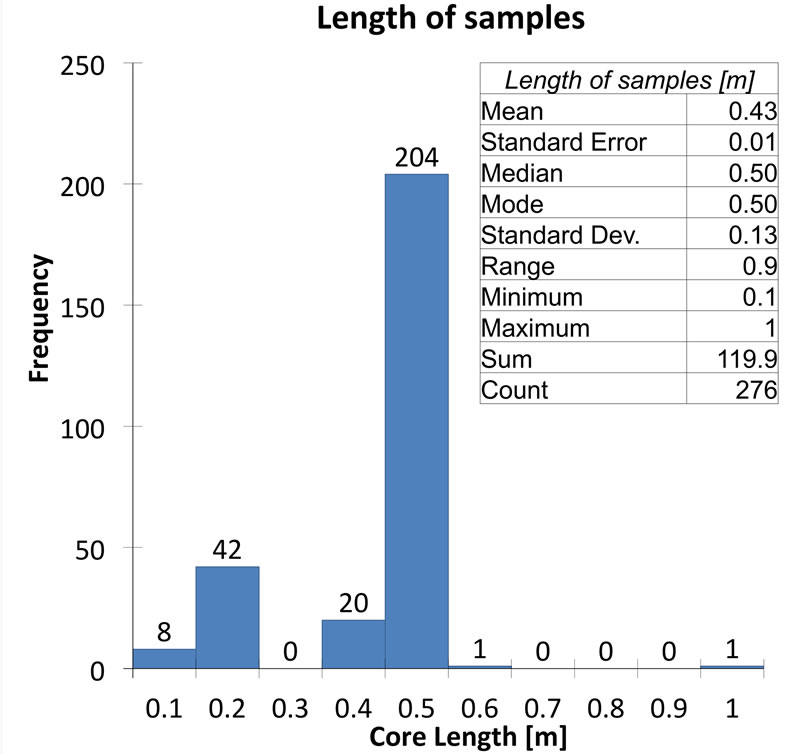
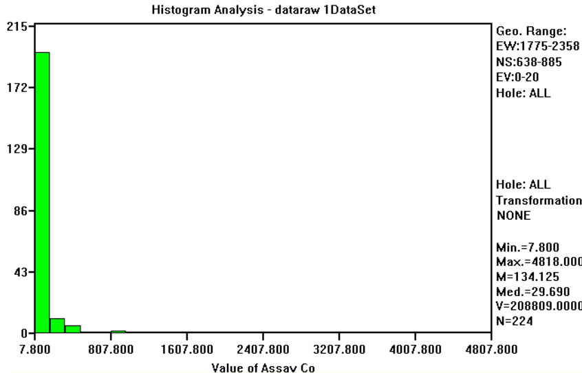
All data measurements are on core samples from the boreholes, the most frequent nearest neighbor distance between them is around 40 m. However, the number of samples per borehole is not constant, as the length of the wells is not constant. In fact, this number varies between a minimum of two and a maximum of seven samples, and on average there are five cores per borehole. There is no obvious pattern in the locations of the boreholes that have the most samples and they are fairly uniformly spread over the study area; moreover, the reason for the differing numbers of sample in boreholes is not known. The length of samples in each borehole varies from a minimum of 0.1 m to a maximum of 1m, as shown by the statistics listed in Figure 2(a) together with the histogram of core lengths.
The lengths of the data gaps caused by these discontinuities are summarized in the histogram and statistics shown in Figure 2(b) which indicate that the lengths of most gaps (i.e. missing data) are either between 0.5 m and 1.5 m, or between 2.5 m and 3.0 m. Figure 2(b) does not give any indication of the locations of the gaps. Most of the 1.5 m gaps are located at a depth of 4.5 m (22.9% of the total number of gaps), and most of the 1.0 m gaps are located at a depth of 2.5 m (20.8%). These observations informed the choice of parameter values in the recomposition procedure.
As the raw data values are measured on unequal sample lengths, the grades must be composited over equal lengths to ensure that all data have the same support.
 (a)
(a)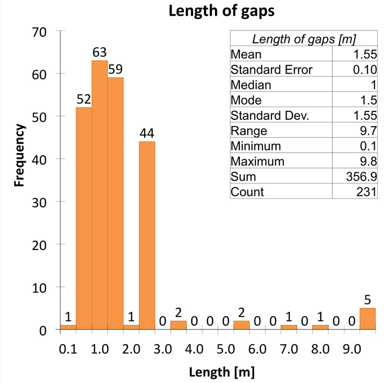 (b)
(b)
Figure 2. Distribution and descriptive statistics of: (a) core lengths; (b) length gaps between sampled cores.
From the histogram in Figure 2(a) a composite length of 0.5 m was chosen, since it appears to be the most representative length, it is an appropriate scale of measurements and minimizes the number of actual sample lengths that are subdivided in the compositing procedure. As additional check on the compositing procedures parameters, the lengths of the raw samples were analyzed in terms of the number with grades exceeding the terrain acceptable concentration limits (TACL) fixed by environmental Italian law [14]. These values may be spatial outliers that could mask the underlying variogram of each variable. As all such lengths are very close to the composite length their influence will not be diluted by compositing to 0.5 m.
Completely, Table 2 summarizes the statistics of the grades of the 50 small-scale (10 cm and 20 cm) samples below 7.4 m. For all variables but the nickel, mean and variance are less than those of the remaining heavy metals and hydrocarbons (HY), and these values could be eliminated from the compositing procedure with negligible effect on any subsequent estimations or simulations. Mean grade and variance of nickel are higher than those of the remaining variables and eliminating these values from the compositing procedure is likely to yield biased estimates and simulations. Introducing the artificial 40 cm and 30 cm samples, as described above, allows these isolated grades of all variables to be included in the compositing procedure.
Totally, the data compositing process yielded 1007 composites from 507 raw splits.
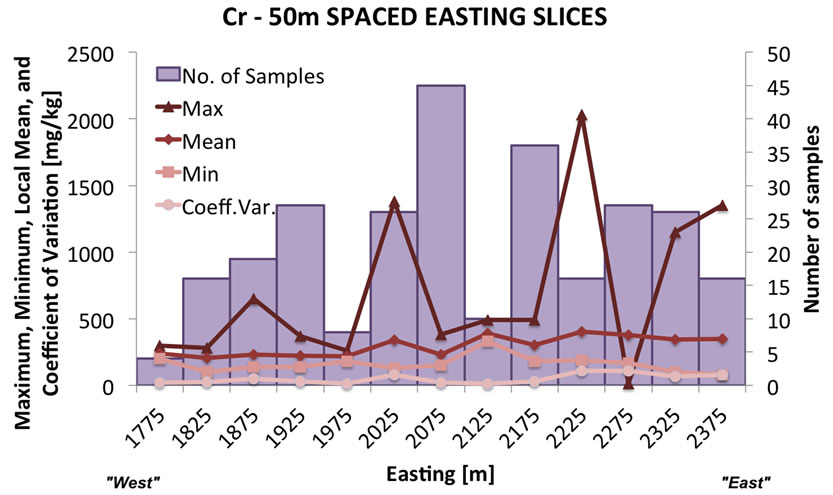
Beside constructing the usual scatter plot maps, the spatial distributions of the data have been analyzed through summary graphs, i.e. histograms of concentration and relative statistics of each variable under study. The histograms of concentration values are based on slicing the three-dimensional soil volume that contains the data and then conducting a statistical analysis of each slice. These slices have been imposed different along the three axes of the space, because the geometry of the volume of contaminated site, in fact the slicing along x-axis from West to East is each 50 m, from North to South along the yaxis the slices are 25 m wide, and from the surface toward the deepest data value the slices are 1 m thick. For each “slice histogram”, one for each main direction of space, some basic statistics are plotted, such as number of samples (bars), minimum, maximum and mean value of concentration, and coefficient of variation (an example is shown in Figure 3).
In general, all the variables show that concentration values in the first depth interval tend to be higher in the eastern part of the study area. Below 2 m the concentration values decrease by increasing depth and higher values tend to be distributed in the central-eastern part. The vertical slice histogram shown in Figure 3(c), Cr concentration decreases quite quickly from the surface and at 10 m it is almost zero mg/kg. This is a logical conesquence of the scarce presence of samples below 10m of depth.
Summary statistics describe numerically the frequency histogram of a variable and provide an initial assessment of the data [15]. The statistics of the 0.5 m composited data are given in Table 3.
The univariate statistical analysis of concentration values shows that all frequency distributions have high positive values of skewness and the mean, the median and the mode are never coincident. These parameters, together with the high value of kurtosis, suggest that the data are not from a Normal (Gaussian) distribution, thus a transform into Gaussian space for sequential Gaussian simulation is necessary. Note that both Co and Ni show less skewed behavior than the other variables. However, even if they are not so skewed, transform in Gaussian space is required. It is assumed that the outliers in this data set are legitimate values. Discarding outliers in environmental applications is not an advisable procedure,
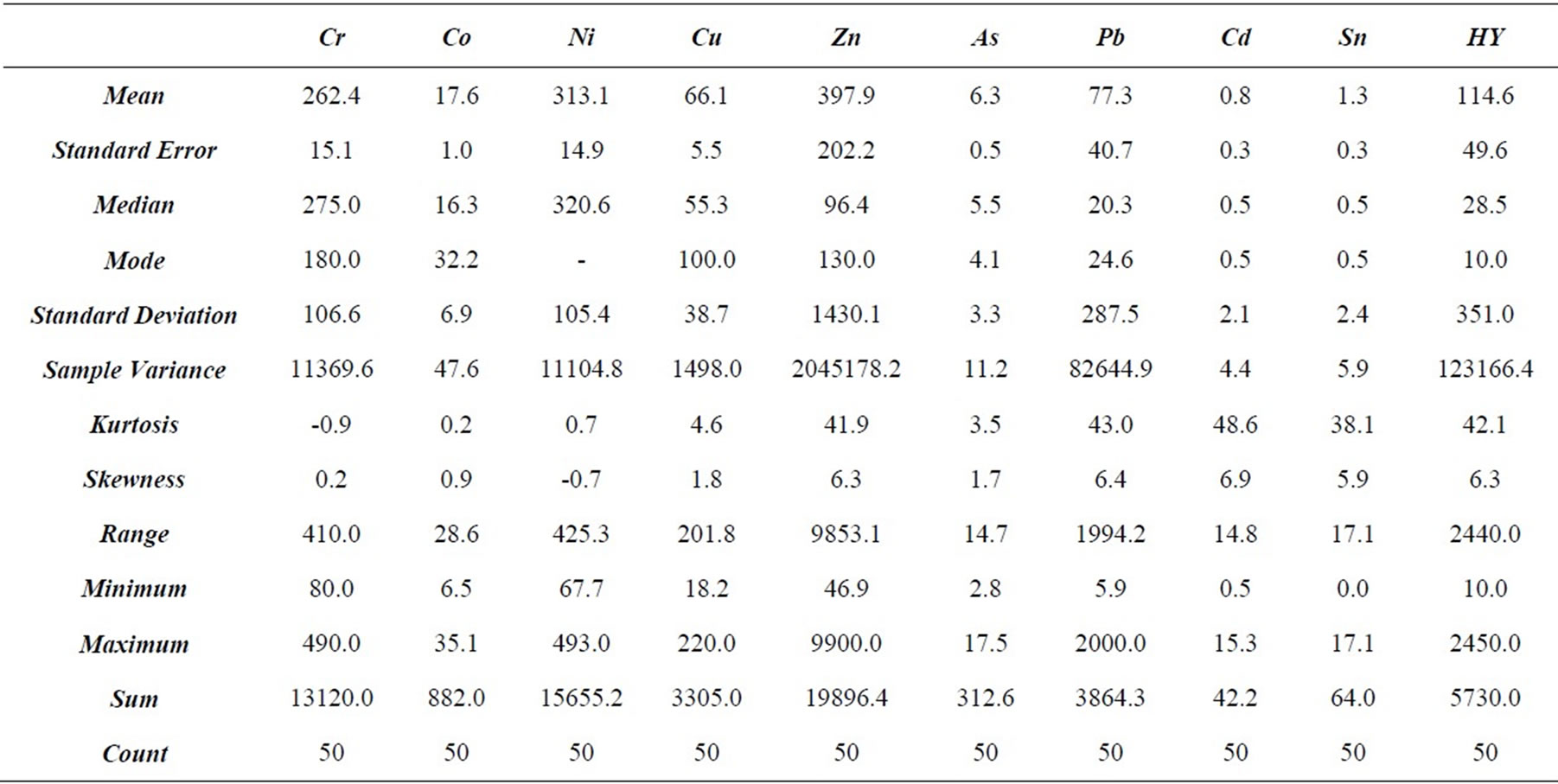
Table 2. Descriptive statistics of data to be eliminated before the recomposition because the short length (unit: mg/kg).
 (a)
(a)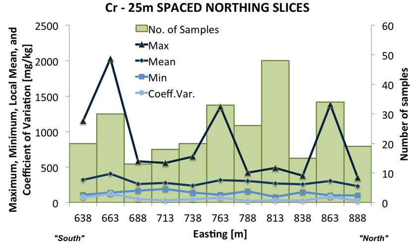 (b)
(b)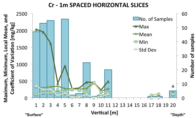 (c)
(c)
Figure 3. Variation of number of samples (bars) and principal descriptive statistics of Cr concentration slicing the site volume: (a) East-West direction; (b) North-South direction; (c) vertical direction.
as these values are of prime concern and interest. Thus the only valid option is data transformation. There are many types of transformation that are used in statistical and geostatistical analyses, including square root of data values, logarithms of the data, a relative transform to the local mean of samples and the Normal scores transform. A normal transform (by normal scores or by some type of a functional form) is also required in this work for the application of the sequential Gaussian simulation method. The data were first assessed for lognormality using the 3-paramenter lognormal distribution [16]. However, assessments for all variables failed and the log-transform option was discarded.
The Normal score data transform is a non-parametric method which is used to transform the data into the Normal space, and to back-transform the data after the estimation and/or simulation calculations [17]. This method does not require the strong mathematical assumptions needed for the log-normal transform. The results, in terms of statistics and normal-probability plots were satisfactory and this method was used for data transformation.
The Normal distribution can be completely defined by mean and standard deviation, which for a standard cumulative density function are zero and one respectively. The transform of experimental z(x) values will generally produce results which approach the Gaussian theoretical ones, but it is unlikely to match exactly the theoretical zero mean and unit standard deviation. Generally, the closer these values are to the theoretical ones, the closer the Gaussian transformed distribution is to the standard Gaussian cumulative density function.
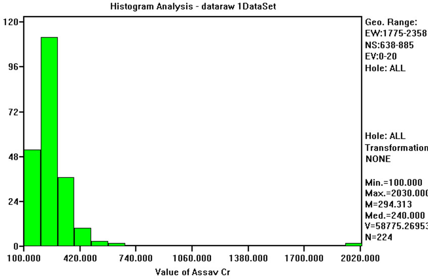
Six on ten studied variables (for instance, Cobalt in Figure 4) have means relatively close to zero and standard deviations close to one. However, four variables (Cr, Cd, Sn and HY) have not so good results. For Cd, Sn and HY this can be explained by the use of a default minimum value equal to the instrumental detection limit. Chromium (Figure 5) is quite well sampled and there are no apparent reasons for these differences, and two or more populations are possible. In fact, the normal-probability curve shown in Figure 5(c) could be approximated by two straight lines, one from cumulative frequencies 0% to 10%, and the other from 50% and 95%. Anyway, this conjecture was not explored any further by fieldwork measures and for all subsequent work it was assumed that the data come from a single population and that the Normal transform is acceptable.
This multivariate data set provides an opportunity to conduct a complete multivariate analysis and further multivariate co-simulations, which can form the basis of a much more realistic risk assessment than a sequence of independent univariate analyses. This observation is, of course, only valid if the two or more of the variables are correlated in situ and/or spatially correlated. Calculating the correlation coefficient matrix, it is possible to assess the correlations between all pairs of variables. From Table 4 the correlations among Cr, Cu, Zn, As, Pb, Cd and Sn are greater than 0.6 and are statistically significant.
Anyway, the correlation coefficient measures only the in situ linear relationship between a pair of variables, but it does not quantify spatial correlation among random variables.
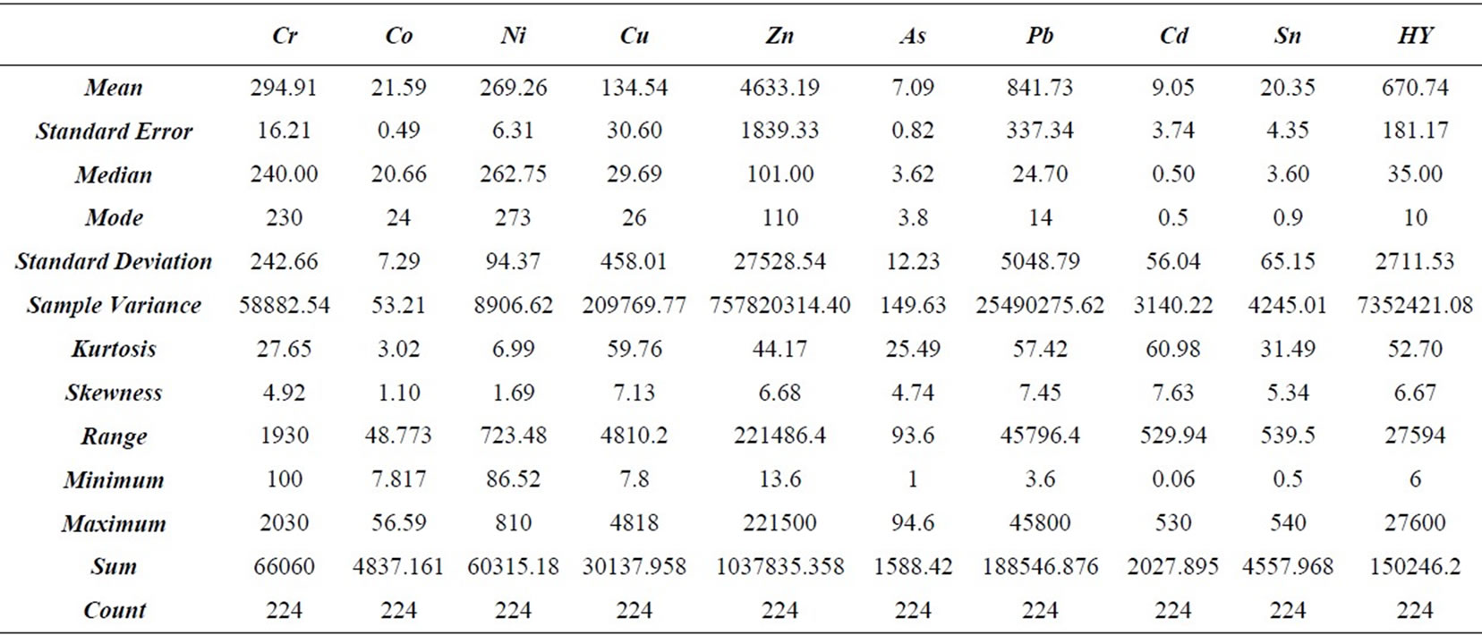
Table 3. Descriptive statistics of 0.5 m composited data (unit: mg/kg).
3.2. Coregionalization
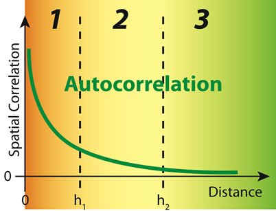
There are two aspects in the study of environmental variables, one is related to the factors determining the values of those variables at any location, and the other is the study of the relatively sample values of these variables. Sample values are viewed as realizations of a random variable drawn from a probability distribution, so at each sample location xi there is a variation from the mean value of that variable. Probability distributions at neighboring locations are, more or less, related with the relationship decreasing with distance between any two locations. Such a variable is generally termed a regionalized variable ([18,19]), which is composed of a random unpredictable component and a structured predictable component. The values of regionalized variables tend to be correlated, and this relation leads to a structure. The spatial correlation among samples generally decreases by increasing the separation distance between them, and may vary in different directions (Figure 6).
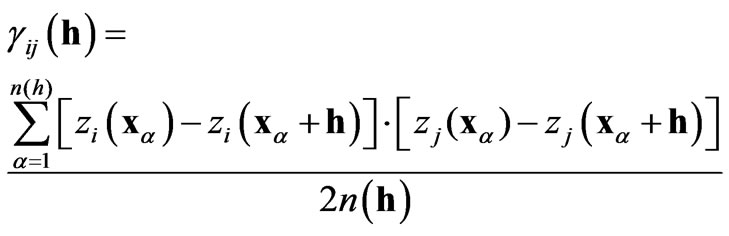
An important tool for the analysis of spatial correlation is the experimental semi-variogram (ESV), which measures the average spatial variability between values separated by a vector h. It can be expressed by the average square difference of each pair of values as follows:
 (1)
(1)
where  and
and  are values of the same regionalized variable separated by the vector h. More details about the semi-variogram and applications can be found in any Geostatistics book (for instance [17,19-22]).
The objective of the structural analysis is to generate ESVs, fit models on them and interpret the models in the context of the local geology and other possible factors conditioning the spatial distribution of pollutants. These models of the variability are then used to simulate realizations of the random variables at unsampled locations. ESVs have been calculated in the horizontal plane for the four main geographical directions and in vertical direction. In addition, omnidirectional ESVs have been calculated. The sparse data provided are characterized by very large variability making it difficult to detect underlying spatial correlation.
The parameters required for calculating the ESV are related to the search pair criteria: lag distance, conical search angle and maximum distance limit [17]. These parameters are used to define orientations for irregular grids. In this study, as the cores are discontinuously sampled in irregularly spaced boreholes, in a 600 m × 250 m area, the lag distance chosen was 40 m, and, a conical search angle of 15˚ was necessary. If this cone extends too far the ESV calculation will average sample values in significantly different directions; so, to prevent this, the cone was bounded by a maximum distance limit of 5 - 15 m.
For vertical variograms the lag distance used varied between 1 m and 2 m, because the most frequent sample distance along a borehole is 0.5 m (in a range of 0.1 m - 9.8 m) and the maximum length of a borehole is 20 m. A lag interval of 1 - 2 m assures a sufficient number of lags in the ESV. As the boreholes are vertical a conical search is meaningless in this direction.
The ESV summarizes the spatial relationships among the data, but it does not describe properly the variance of the regionalized variable, because each particular lag is exclusively an evaluation of the mean semi-variance for that lag and is subject to sampling variability, which in-
 (a)
(a)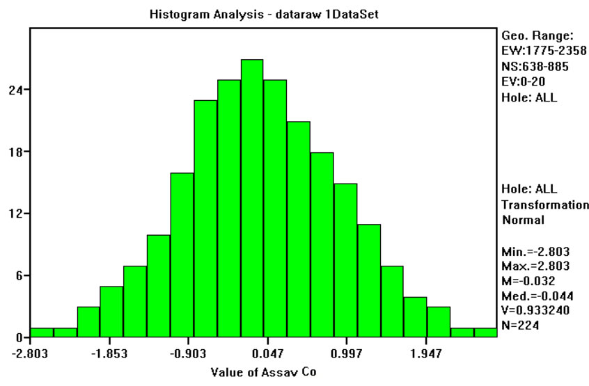 (b)
(b)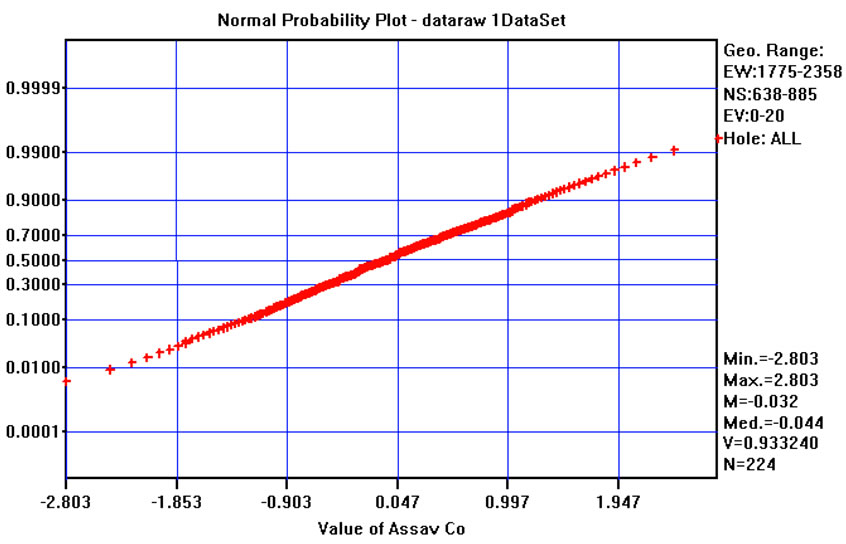 (c)
(c)
Figure 4. (a) Frequency distribution of Co raw values; (b) Frequency distribution of Normal Scores transformed values of Co; (c) normal-probability plot of normal scores transformed values of Co.
creases as the number of samples decreases, and it is interpolated by a model, i.e. a mathematical function defined for all real distance h, which is used in both estimation and simulation procedures.
The variogram model is completely defined by its parameters: the type of mathematical function adopted (the model γ(h)); the behavior near the origin and the positive
 (a)
(a)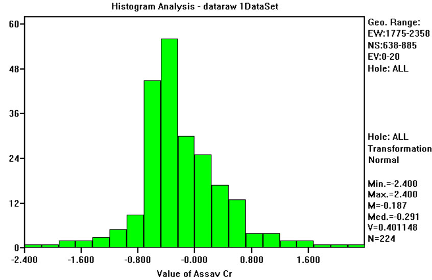 (b)
(b)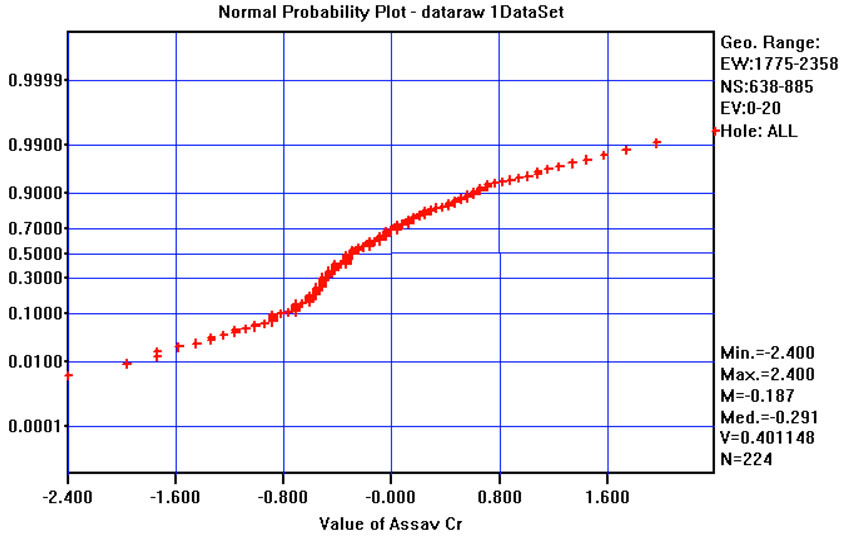 (c)
(c)
Figure 5. (a) Frequency distribution of Cr raw values; (b) Frequency distribution of Normal Scores transformed values of Cr; (c) normal-probability plot of normal scores transformed values of Cr.
intercept on the ordinate (the nugget variance C0); the range of the variogram (or autocorrelation distance) that changes with direction if there is anisotropy, and from which the curve reaches a constant maximum or an asymptotic value (the sill Ci) [21].
The ESVs were not modeled independently of each other and several attempts were made to find a valid linear
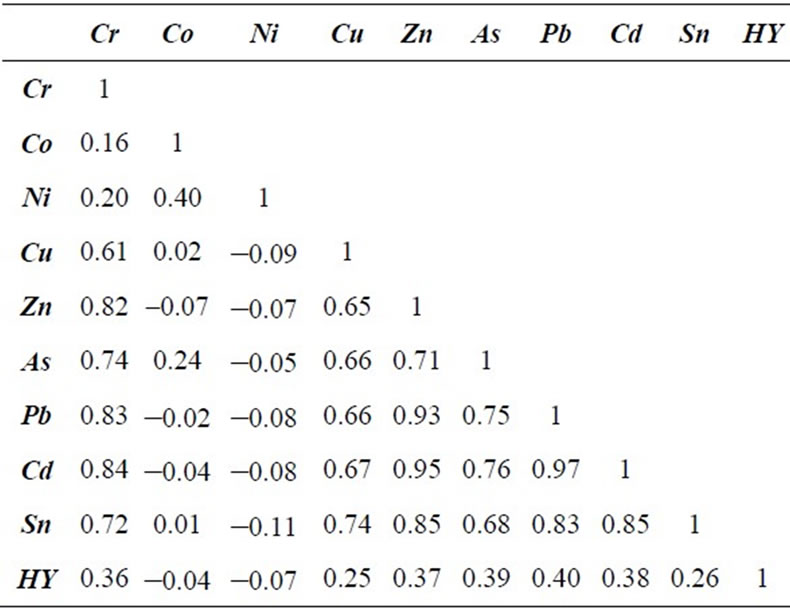
Table 4. Correlation coefficients matrix of raw recomposited data (highlighted cells in this table represent the absolute values of correlation coefficient greater than 0.5).
 (a)
(a)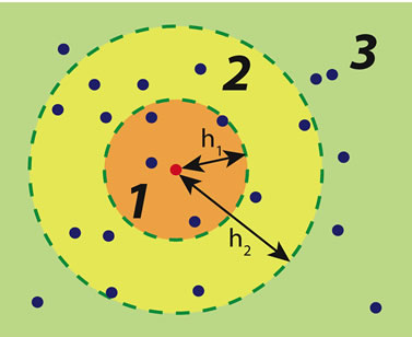 (b)
(b)
Figure 6. Spatial auto-correlation: (a) example sampling map and relationships between a sample with the other sampled localizations in three distance classes; (b) empirical relationships between spatial correlation vs distance.
model of coregionalization, which requires the same range for each directional ESV for each variable. This was an iterative procedure that started from a rough fitting of the ESV by a simple model for each variable. The models were validated by means of cross-validation and then the parameters of each model were adjusted to achieve a balance between the requirements of a positive-definite linear coregionalization model and the need for the variogram models to reflect the behavior of the ESVs.
By definition, the linear model of coregionalization is a sum of proportional covariance models [21]. Proportional covariance models are models in which all covariances (or all variograms) are proportional to the same covariance (or variogram) function [20]. The variables
 are considered to be a linear combination of
  independent variables with covariance
 , and expressed as follows:
 (2)
(2)
The variables  are inter-correlated with crosscovariances given by:
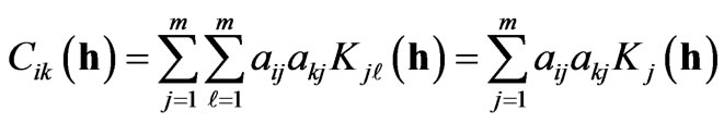 (3)
(3)
or, either in terms of variograms or in matrix form:
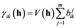 or
or 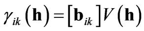 (4)
(4)
where [bik] is the positive definite matrix of symmetric coefficients bik. The positive definiteness of these matrices is achieved by checking that the eigenvalues of each matrix are real and positive. The structural part of the variogram (i.e. V(h)) remains the same for every coefficient. This is the reason for which all variograms and cross-variograms have the same range in a particular direction.
There are automatic procedures that can fit linear models of coregionalization among whatsoever number of variograms and cross-variograms. However, like other automatic procedures, there is no guarantee that they will work properly in all applications. In such cases manual adjustments of the fitted models are needed. Two problems were encountered in the manual adjustment of parameters in this project:
• Fixed range of anisotropy in any direction;
• Assumption of positive definite variance-covariance matrix.
Often, if the ESV was to be respected, the range of possible values for adjusting parameters was very narrow, and even small changes in values contravened the positive definiteness requirements. A linear model of coregionalization was fitted (or at least refined) by trial and error.
The models comprise two structures: a nugget variance (C0) and one nested spherical structure (C1) with three different range of anisotropy. The ESV identifies the anisotropic behavior of the variables, even though it is difficult to detect this from the raw data. The axes of the anisotropy ellipsoid are: E-W direction (aNS) = 130 m; N-S direction (aEW) = 80 m; Vertical direction (aVert) = 6 m. The vertical range might be limited by the maximum length (20 m) of the boreholes. It is unlikely, however, that the high levels of contamination in the first few meters are related to the low values of concentration at depths below 10 m (see for instance); it is also unlikely that very high values of concentration will be found in deeper samples if and when they are collected. Thus, the vertical range found in this study for the first nested spherical structure C1 would probably not change with additional deeper sampling but it is possible that such sampling might reveal an additional longer-range structure. This is because deeper samples are likely to reflect the natural background concentrations of the variables.
As there are nine heavy metals variables above the TCAL, the next step is to assess spatial covariability among the variables. One variable can be spatially related with another in the sense that its values are spatially correlated with the values of the other variable. This inter-correlation among variables should be included in any realistic simulation of pollutant concentrations, especially when they are genetically similar, like in this case study (all variables are metals). This concept forms part of the general principle of coregionalization [22].
A tool for studying coregionalizations between two regionalized variables  and
and  is the cross-semivariogram or, more simply, the cross-variogram
 , which describes the spatial variability between
  and
and  with increasing distance between samples. The experimental cross semi-variogram (X-ESV) is calculated as follows:
 (5)
(5)
where  and
and  are values of the same regionalized variable
  separated by the vector h, and
  and
and  are values of the same regionalized variable
  separated by the same vector h [17]. The cross-variogram is a measure of the variability of two variables at the same locations.
X-ESV is symmetric and can be calculated only for the locations where there are values of both variables. In this project, the variables under study have not been measured in the same way everywhere, so crossvariograms can be calculated just in some locations. X-ESV can be modeled in the same way as variograms using the same types of models. The only inconvenient is that cross-variograms must be calculated for every possible pair of variables: in particular for this project, nine ESVs and 39 cross-variograms must be calculated, modeled and adjusted to conform to a linear coregionalization model together with direct variograms (ESVs) defined by the anisotropic structures (same range for all ESVs and X-ESVs). The two structures, C0 and C1, fitted to each experimental variograms and cross-variogram are listed in Tables 5(a) and (b). In these tables the variance components of each direct variogram are highlighted. The respective eigenvalues are also listed in both of tables, because they define the real positive condition of this matrix, mandatory constriction for establishing a linear coregionalization model. For most X-ESVs the two structures are positive and only al pairs where Ni is present and some variables pairs where C0 is present have negative X-ESVs’ trend. This agrees with the correlation coefficients shown in Table 4.
Note that C0 generally contributes significantly more than C1 to the total covariance (upper triangle in Table 5(a)). This randomized background noise may indicate that there is a very short-range structure, which is not detected by the data because of the sampling configuretion and sampling grid.
Upper triangle in Table 5(a) provides a quicker way of understanding how the random component affects the spatial correlation modeled between each pair of variables. On average in this case study, the C0 component contributes around 50% to the total variability (C0 + C1) and sometimes it is the only significant component, e.g. for the cross-variograms for Ni-Co, Ni-Zn or Ni-Pb. This implies that Ni is not significantly spatially correlated with the other variables in the study area, because there is almost a complete absence of structure in most of the cross-variograms in which it appears. On the other hand, Cr, Co, Zn, Pb, which are highly correlated each other, and highly spatially correlated too in terms of crossvariograms.
Given the large number of cross-variograms produced, only a few examples are given here in Figure 7. Considering the pair Zn-Pb, horizontal cross-variograms show good structure (Figure 7(b)), even though the anisotropy is not so evident. The vertical cross-variogram for the same pair shows some structure up to the range of 6m (Figure 7(d)).
Cross-Validation is a back estimation technique for testing different variogram models fitted to an ESV and X-ESV, providing comparisons between the actual value z at each sampled location  and the (kriged) estimated value
 . It is a powerful method of validation to check the performance of the variogram model for kriging [20]. Performing this procedure, the mean standard error should ideally be equal to zero, and the standard deviation of the estimation errors, when standardized by dividing by the square root of the kriging variance, should be 1.0, that means in the ideal case the error distribution tends to be similar to the parameters corresponding to the standard Gaussian distribution.
In this project, none of the above conditions were theoretically respected. However, the variogram models were considered validated after several iterations of crossvalidation and refining the model parameters. So, the variogram parameters entered for the cross-validation satisfy the requirements of a linear coregionalization model.
Factors affecting the coregionalization can be related to the general geological and hydrological sketches. The vertical range of 6m may represent the average thickness of Unit 0, i.e. the backfill material. Generally, this mate-
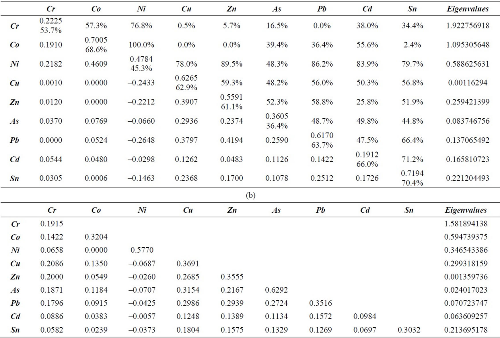
Table 5. Matrices of linear coregionalization model fitted and respective eigenvalues: (a) structure C0, or nugget effect (lower triangle and first value in diagonal’s cells), and percentage contribution of C0 to the total variance (C0 + C1) for ESV (second value in diagonal’s cells) and X-ESV model of each variables pairs (upper triangle; (b) structure C1, sill of spherical structure.
rial comprises industrial waste and is spread almost everywhere over the study area to a depth of approximately 4 m. It is, however, unlikely that the metals do not penetrate at least a further two meters below this unit. Furthermore, lenses of different materials can be detected over the entire area at depths of 5 - 6 m. These lenses are composed of gravely sand and/or silty sand, inside a thicker volume of pebbly gravel. Vertical cross-sections in Figure 1) show a succession of three different materials in the first 6 m and three more types of material between depths of 6 m and 12 m. This should explain the generally well-defined 6 m range on the vertical variograms and cross-variograms.
The range of variograms is 130m in the E-W direction and 80 m in the N-S direction, implying some type of geological structure, or succession of levels, which is more continuous in the E-W direction than in the N-S direction. One possible explanation for the major axis of the anisotropy ellipsoid in the E-W direction is related to the several lenses of different material included in a larger and more homogeneous volume. These lenses could be the remainder of meanders of some small tributary stream of the Po River, or the residual of a small, local alluvial event in the quaternary period rather than a stream. There are, however, no indications of a meander or channel in the cross-sections provided for this study.
The major range of anisotropy (E-W) can be related to the main flow direction of the stream in this area. Slopes tend to decrease from East to West, toward the major stream, the Po River. Thus, the tributary streams, the meander and the alluvial event tend to be more extended in the E-W direction than in the N-S direction. Thus, a plausible interpretation of the E-W and N-S ranges is that they reflect a quasi-random dispersion of long and relatively narrow lenses of different material.
Another explanation could be based on geochemistry considerations. The slice histograms (example in Figure 3) show that there are almost always concentrations are extremely high in the first 2 - 3 m and then decrease very quickly down to a depth of 5 - 6 m, below which there is a relatively low, homogeneous concentration. The vertical variogram should reflect this aspect. Indeed the first lags
 (a)
(a)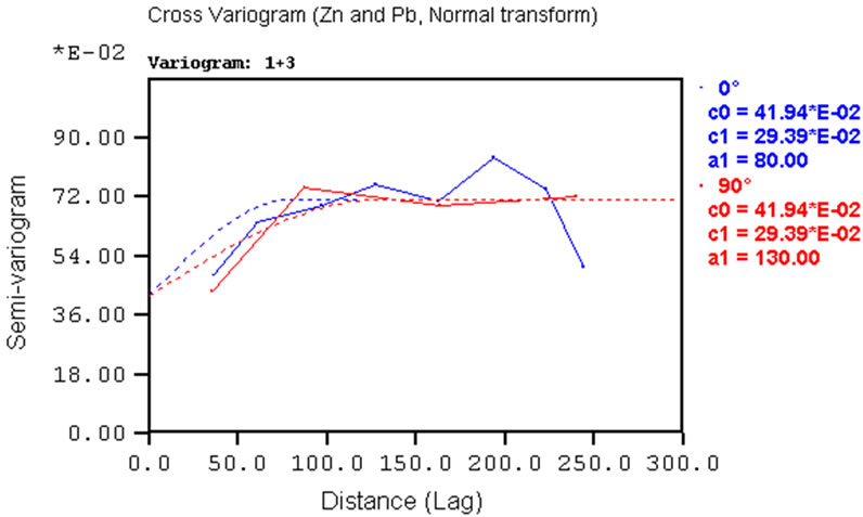 (b)
(b)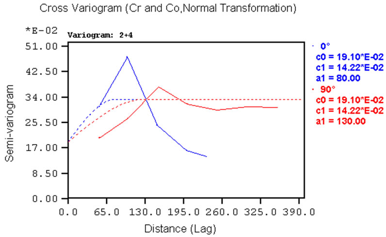 (c)
(c)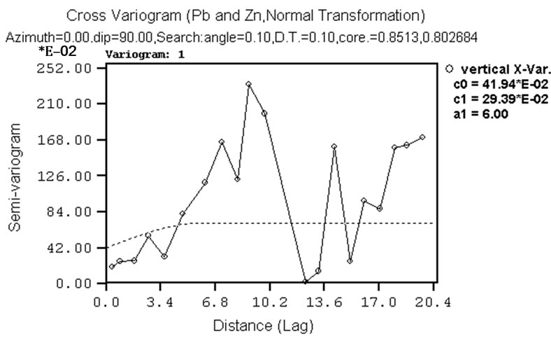 (d)
(d)
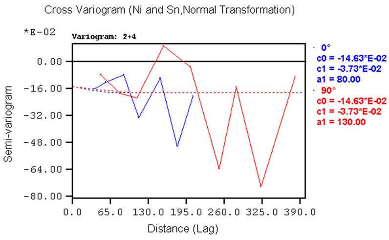
Figure 7. Examples of experimental cross-variograms and models for variables pairs: (a) Ni-Sn; (b) Pb-Zn; (c) Cr-Co. Example of vertical experimental cross-variograms and models for Pb-Zn variables pairs.
show good correlation up to 6 m, after which spatial correlation decreases and becomes erratic, implying that almost everywhere there are strong relationships between the closer samples.
Moreover, as the coefficient of permeability is quite high in the first geological units, the contaminants tend to be dispersed along the main groundwater flow direction, which is gently sloping from East to West. This could explain why the narrow dimension of the anisotropy ellipse is oriented in the East-West direction.
3.3. Simulations
The objective of geostatistical simulation is to provide alternate realizations of regionalized variables on any specified scale ([17,19,20]). It does not create data but provides a possible reality at unsampled locations. Estimation algorithms tend to smooth the spatial variation of a variable; in particular they overestimate small values and underestimate large values. This complicates to detect patterns of extreme high values, for instance metal concentrations above TACL. Moreover, the estimation smoothing effect is not the same everywhere as it depends on the data configuration and it will be low for dense samples. A smooth interpolator should not be used for applications in which the pattern of continuity of extremely high values is critical [17]. Geostatistical simulation can be applied to the assessment of the variability of a regionalized variable and the quantification of the uncertainty associated with the value of a regionalized variable sampled at specified locations.
Once the contaminants of the volume have been simulated, the volume can be subjected to any number of simulated operational activities and it can be used to assess the likely concentration of a metal above the law limit [1]. Moreover, remediation projects can be designed on the basis of the sampled data and the results compared with the simulated “reality” of the variable.
Following the initial Turning Bands Method many other geostatistical simulation techniques have been developed [23]. The choice of one method over another is based essentially on the application. For this project sequential conditional methods were chosen. These techniques are easy to implement and provide a simple, robust and manageable implementation. The do, however, requires a few assumptions [24]. A simulation in which the simulated values coincide with the actual data (or conditioning) values at the sampled locations is termed a conditional simulation and meets the following criteria:
• They coincide with the actual values at all data locations;
• They have the same spatial correlations, i.e. the same variogram, as the data values;
• They have the same distribution as the data values;
• They are coregionalized with other variables in the same way as the data.
• Two different methods of geostatistical simulation have been implemented in this project:
• Correlation correction of univariate Sequential Gaussian Simulations;
• Sequential Gaussian Co-Simulations.
3.3.1. Correlation Correction of Univariate Sequential Gaussian Simulations
Sequential Gaussian Simulation is a direct conditioning method of simulation ([23,25]). It is principally a data driven technique and is only valid for multi-Gaussian random variables. The main steps of the procedure are:
1) Transform data to standard Gaussian values (conditioning data);
2) Calculate the ESV of conditioning normal transformed data, then fit and validate a model;
3) Define a random path through all grid points (grid nodes) to be simulated;
4) Choose a simulation grid node and krige the value at that point using conditioning data and all previously simulated values;
5) Draw a value for the grid node from a normal distribution having the estimated kriging value as mean and the kriging variance as variance;
6) Add this point to the conditioning data as a realizetion of the random variable and include it in kriging the value at all subsequent grid nodes;
7) Repeat steps 4 - 7 until all grid nodes have been visited;
8) Take the inverse transform of the Gaussian conditionally simulated values;
9) Correlation correction of univariate simulations.
The basic assumption and the only apparent limitation of SGS is that it works with intermediary Gaussian distribution. So, the normal transformed variables  must follow a multi-Gaussian distribution. As it is impossible to check whether these variables are multiGaussian, the verification is limited to checking for univariate and bivariate normality.
A test for a bi-variate Gaussian distribution can be performed by means of h-scatter plots, which plot all the pairs of measurements of the same attribute z at locations separated by a constant distance  in a given direction. The shape of the cloud of points on the h-scatter plot indicates whether there is any correlation between adjacent z values [17].
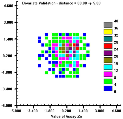
A bi-Gaussian distribution will plot as an approximate spherical cloud of points. So, h-scatter plots were plotted for three different distances (30 m, 50 m and 80 m) for each variable (an example is given in Figure 8 for Zn). This visual checking was performed for all variables, and in practice all of them satisfy the bivariate normal requirement, from which it could be conjectured the multivariate Gaussian condition. For each variable, 500 simulations were generated. SGS was used to simulate realizations of regionalized variables at each node of a regular three-dimensional grid (voxel size: 5 m × 5 m × 1 m; No. voxel: 130 × 75 × 22) that included all conditioning points, i.e. all samples The composited data were used for SGS. However this introduces more uncertainty into the simulation, because of the isolated shortest samples, adjacent unsampled lengths were added to the dataset with grades equal to mean grades of each variable. Both kriging and variogram model parameters are the same as those used to define the linear coregionalization model and to do the cross-validation, and they will not berepeated here. The only difference is the number of previously simulated points that must be used in kriging
 (a)
(a)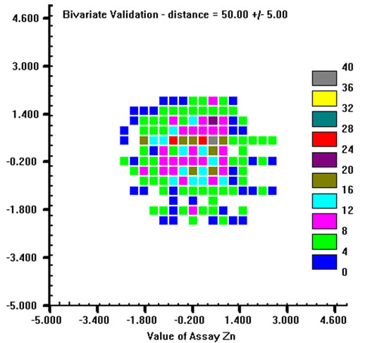 (b)
(b)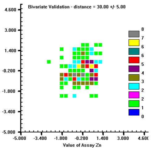 (c)
(c)
Figure 8. H-scatter plots for Zn at (a): 30 m, (b): 50 m, (c): 80 m distances.
each new simulation grid node. This number was set equal to the maximum number of conditioning data to be used in kriging within the imposed search radius.
After simulating, a back transform to the original sample space was automatically performed. The linear extrapolation method was used to deal with the upper and lower tails of the Gaussian distribution, i.e. it was assumed that the values in the lower and upper tails follow a uniform distribution [10]. As the simulation was done for blocks, the volume has been sliced for visualizeing the simulation before validating it. For instance, comparing the map in Figure 9 with the row sampled As data, it is obvious that the higher data and simulated values are in roughly the same position.
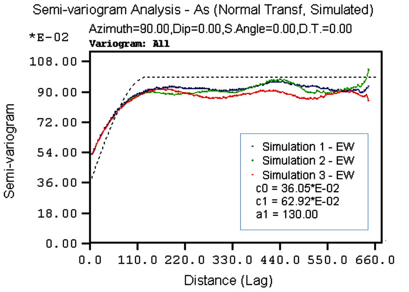
However, the common way of validating simulation results is via descriptive statistics and the spatial variation of the simulated values in comparison to the conditioning data. Descriptive statistics, frequency distribution, normal-probability plot, and variograms have been calculated for all variables. The frequency distributions of the back-transformed simulated values for all variables reproduce the raw data histograms, although the former are slightly less variable than the latter. The normalprobability plots of the Gaussian simulated values reproduces that of the normal transformed conditioning data. As the variogram modeling was done in the Gaussian space, the variograms were validated by comparing the ESV of the simulated normal scores values with the (input) variogram models fitted to the normal transformed conditioning data. By way of example, Figure 10 shows the validation for As variable, three different univariate simulations and the spherical model deriving from the linear model of coregionalization for the EW, NS and vertical directions are shown. The reproduction of the variograms is satisfactory in the three major directions of the space. In general the ESV for all simulated variables tends to show a higher nugget variance and a slightly longer range than the corresponding parameters of the specified model. This could be caused by the presence of the extremely high values in the shallower
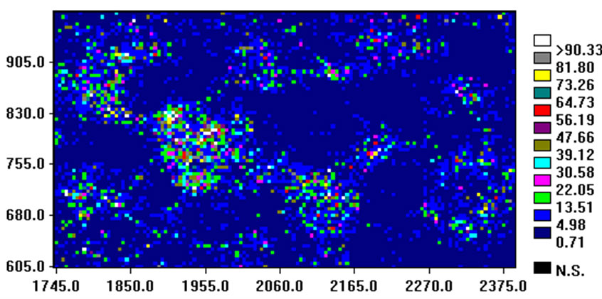
Figure 9. Example of three-dimensional SGS result for AS (legend unit: mg/kg): horizontal cross-section at 3 m below the surface.
 (a)
(a)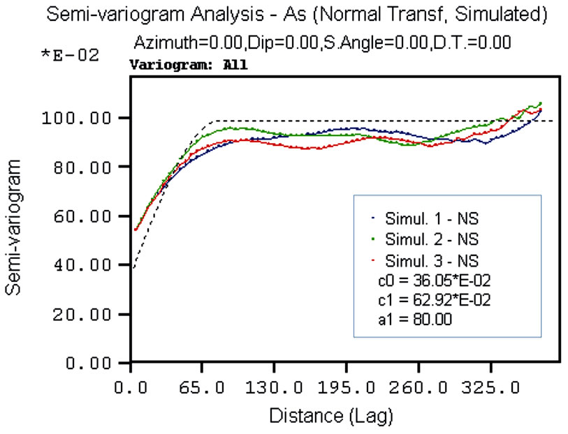 (b)
(b)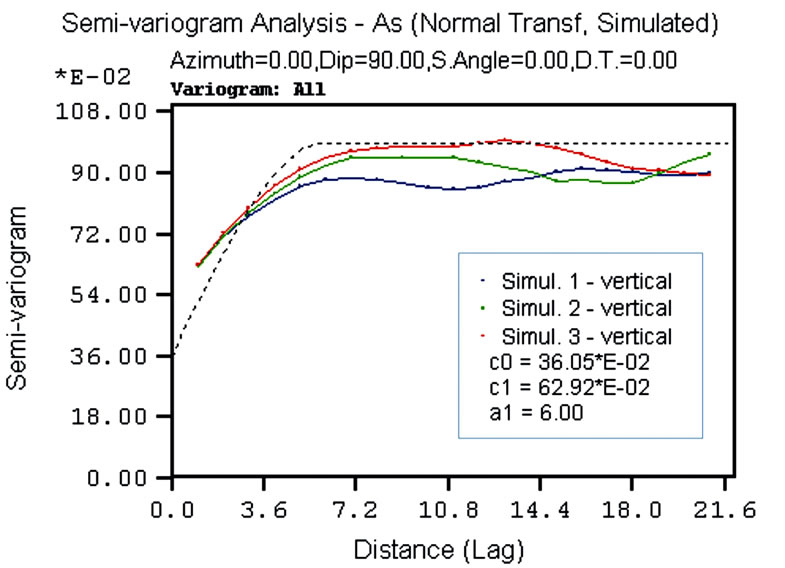 (c)
(c)
Figure 10. Simulation results of As ESV and imposed variogram model for: (a) EW direction; (b) NS direction; (c) vertical direction.
levels, surrounded by low values. SGS is a data driven method and any structure implicit in the data will tend to enforce precedence over the specified model. In terms of the variograms the simulations are deemed acceptable.
Correlation correction method simplifies the co-simulation by using directly the univariate SGS results to introduce correlation among the simulated values. In a multivariate Gaussian context, if all covariances are proportional, the co-simulation by parallel simulations combines the variables linearly to impose specified correlations among them [20].
Multivariate datasets are common in environmental applications and generally these variables are negatively or positively correlated. The “Variable Correlation Correction” module of GeostatWinÔ software [10] allowed to impose the specified correlations on the independently simulated variables. The only limitation of this software is that it can handle a maximum of five variables and so the most highly correlated variables were chosen, i.e. Cr, Zn, As, Pb, and Sn.
The variable correlation correction procedure can be applied to both generic simulated variables and correlated simulated variables. However, univariate simulations performed by SGS are not correlated before imposing this correlation correction. The correlation coefficients of the back-transformed simulated values are less than 0.1, so there is not “a priori” correlation (Table 6).
The correction was made by imposing the correlation coefficients of the raw conditioning data and performed in the Gaussian space, and than back-transformed to the sample data space.
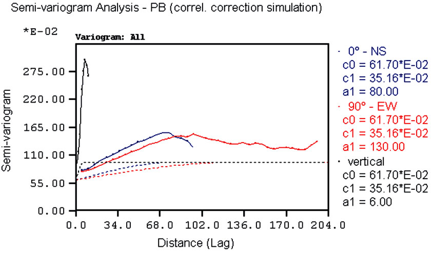
The correlation correction simulations reproduce the conditioning distribution although the former is slightly smoother than the latter. From the variography these corrected simulations display higher spatial variability than the uncorrected simulations. By way of example, variograms for the corrected simulations of lead and zinc are shown in Figure 11, from which it can be seen that the directional variogram models are consistently lower in all directions, especially for the vertical direction. Furthermore, the ranges of corrected simulated values are generally shorter than those of the linear coregion-alization model.
Comparing these variograms with those of the uncorkrected SGS (Figure 10) it is evident that the latter produce better results in terms of spatial variability (better
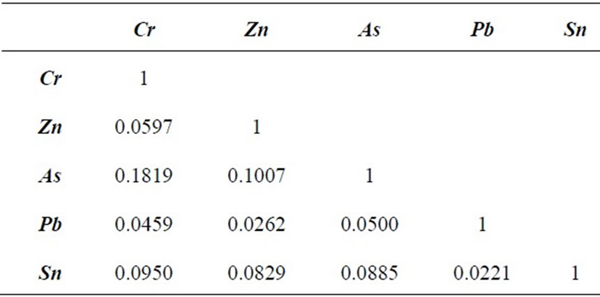
Table 6. Correlation coefficient for back-transformed simulated values of five variables to be corrected.
 (a)
(a)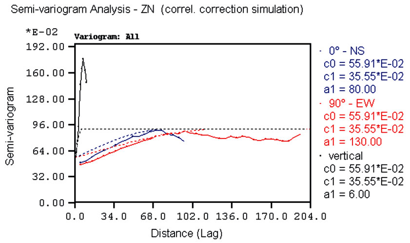 (b)
(b)
Figure 11. ESVs of simulation managed by correlation correction: (a) lead; (b) zinc.
fitting) so the correction increased the simulation efficiency.
3.3.2. Sequential Gaussian Co-Simulation (SGCOS)
SGCOS is essentially a direct conditioning method of simulation which takes into account the spatial correlation among a set of regionalized variables by using the parameters of a linear coregionalization model [21]. It is essentially a data driven technique valid for multi-Gaussian random variables and is very similar to SGS, except that kriging is replaced by cokriging for estimating any single node to be simulated. The drawbacks for this method is the difficult in finding the same range of anisotropies, the significant increasing in computing time over SGS, and it is more effective for two or three variables and a relatively small dataset [10]. This step of the project was conducted in the Gaussian space using the Geovariance ISATIS software [26].
For each variable, five co-simulations were generated. As performed for SGS simulations, also the co-simuations were validated by comparing the frequency distributions of simulated values with those of the normal transformed conditioning data for all variables together with the normal-probability plots. The simulated values respect the distributions of the actual values, although the former are slightly smoother than the latter.
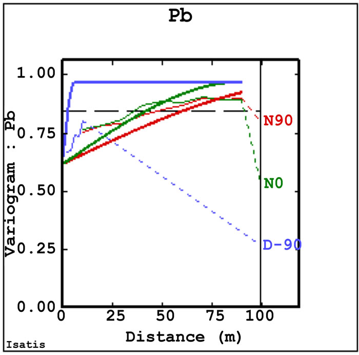
Spatial structures were validated by comparing the variograms and cross-variograms of the co-simulated values with those of the conditioning data. By way of example, Figure 12 shows two direct variograms and two cross-variograms. These are just an example of the total of nine direct variograms and 36 cross-variograms produced for the linear coregionalization model established among the heavy metals variables. Note also that these variograms relate to only one simulation. Five hundreds simulations were generated and a complete validation would include variogram and cross-variogram synoptic comparisons for all simulations.
The horizontal direct variograms (Figures 12(a) and (b)) reproduce the linear coregionalization model quite well. The ESVs of co-simulated values have generally higher nugget variance, but they have the same ranges and sill values of the linear coregionalization model of the conditioning data. For the vertical direction the direct ESVs for each variable are differ from the theoretical coregionalization model, but tend to have the same range.
Almost every cross-variogram between tin and any other variable does not match the coregionalization model. Low cross-correlation is also shown for nickel and arsenic. On the other hand the cross-variograms for cobalt and all other variables reproduce the coregionalization model.
In conclusion, SGCOS (an example is shown in Figure 13) can improve the simulation of high statistically and spatially correlated regionalized variables but for moderate to low correlations the co-simulation procedure does not improve the results regarding to the correlation
 (a)
(a)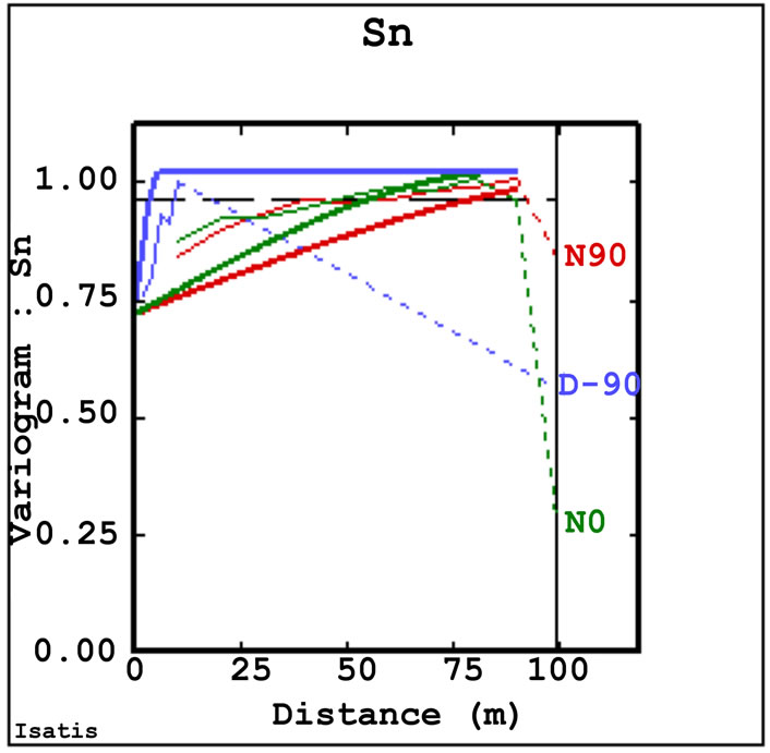 (b)
(b)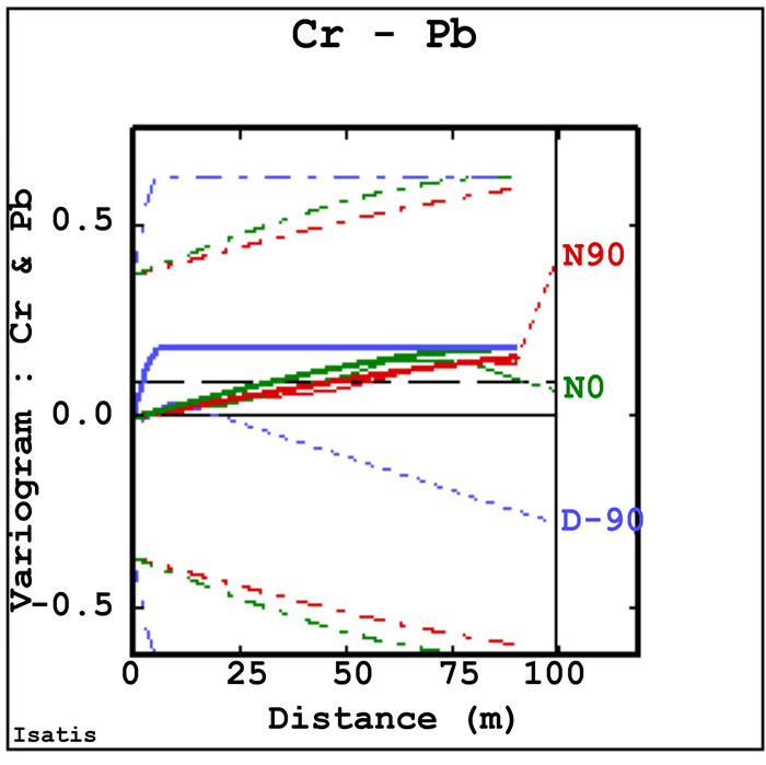 (c)
(c)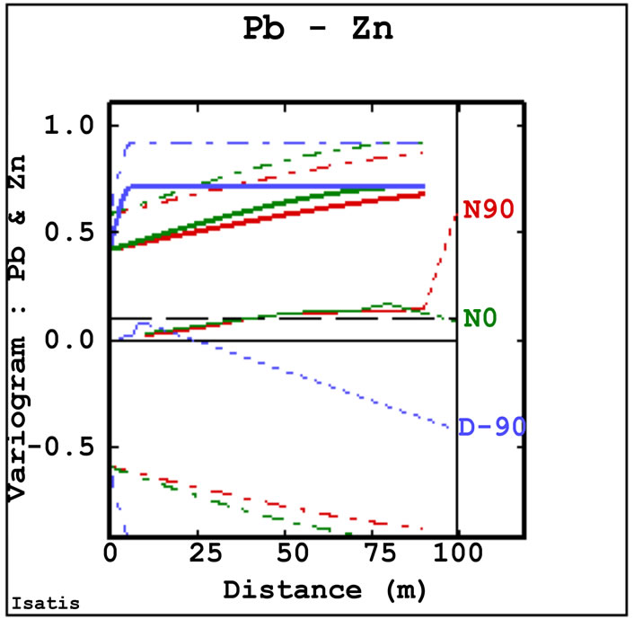 (d)
(d)
Figure 12. Example of direct variograms and cross-variograms (thin lines) and respective models (thick lines) for co-simulated values, together with the boundary of positive definition of the model (dashed lines).
correction of univariate simulations.
4. Risk Analysis
Risk is a measure of the probability and severity of adverse or unexpected effects, whereas safety is the degree to which risks are judged acceptable. Risks can be distributed over part of a population or over geographical areas and these distributions may be more important than the magnitude of the risk itself [1]. Diffuse risks of contamination by inorganic compounds slightly above acceptable limits, but over large areas, may affect the population more than rare high concentrations in localized zones. The acceptability of risk is determined for a particular area by technical considerations and/or political law on the basis of quantified risk.
A percentage of risk is always present and cannot be removed. So, the best way of dealing with the risk is to reduce it to the minimum by identifying, assessing and identifying the risk, determining the minimum acceptable level of risk, reducing the risk to the minimum and, finally, managing the residual risk [1].
In general, realistic quantification of risk requires adequate models of the processes causing risk. The acceptability of risk is determined by risk-benefit analyses, i.e. by analyzing whether the benefit is worth the residual risk. In the case of a contaminated site, this benefit could be measured by the cost of a remediation project in relation to the further industrial use of the site. The benefit depends on whether the site is used as a new comercial/ industrial site, rather than new urbanization area. For the latter case the decision-maker must take into account more restrictive parameters in risk-benefit analysis.
Ultimately, quantified risk analysis requires an estimate of the likelihood of an event occurring. This quantification can be done by geostatistical simulation for a given variable over a studied volume. Risk can be asessed by repeating simulations and generating additional images of possible realities. The greater the number of simulations is, the more accurate the risk quantification will be. A curve showing the concentration (grade) and tonnage of a particular contaminant is a simple way of assessing the probability that the contaminant will exceed acceptable limits. A realistic risk analysis must be based on block tonnages and grades estimated from the ‘sample’ obtained by ‘drilling’ the simulated volume to
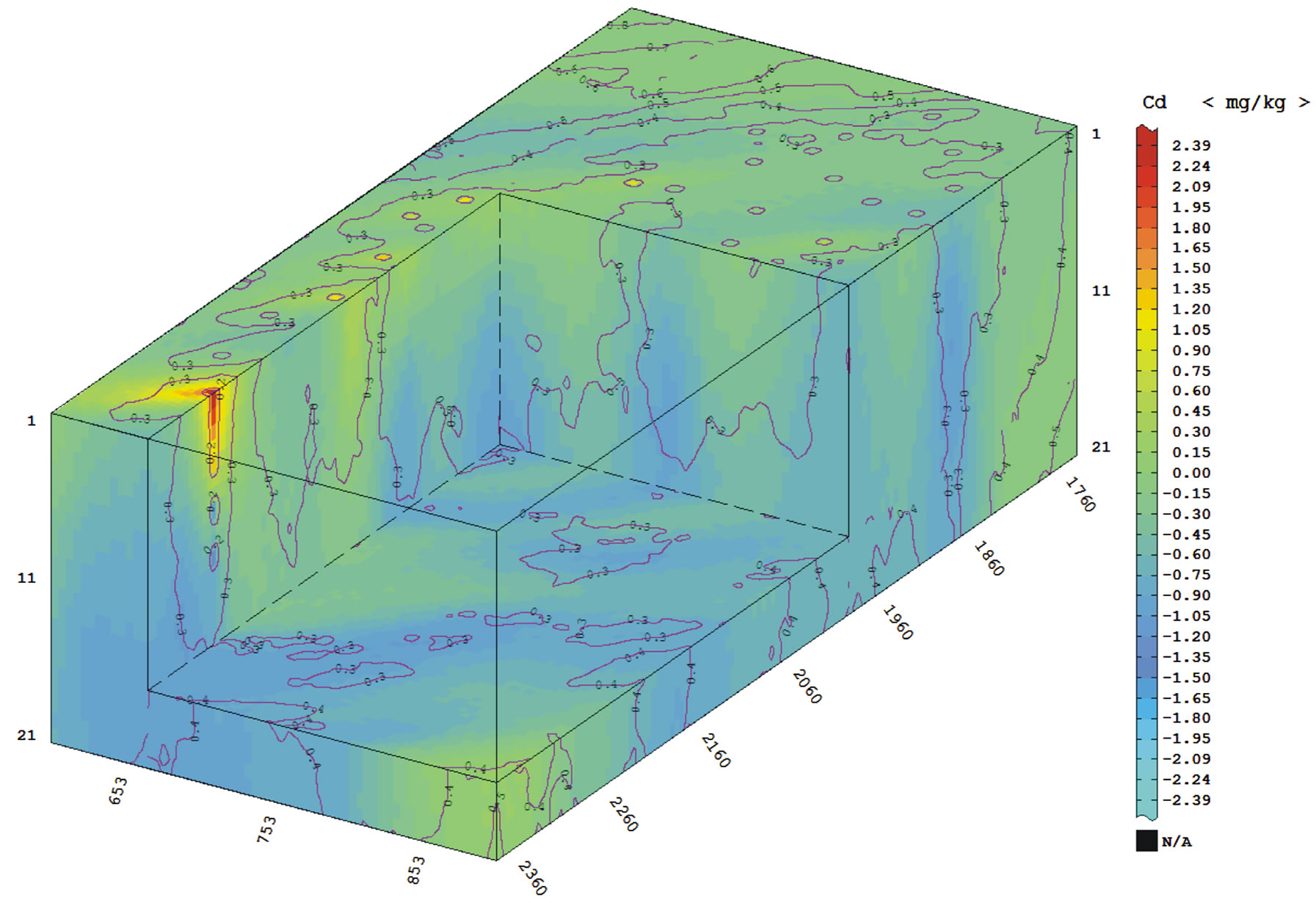
Figure 13. Three-dimensional representation of the mean of 500 SGCOS results for Cd variable (color ramp) and standard deviation for simulation (isolines).
be subjected to remediation [1].
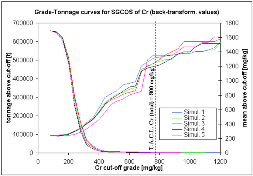
Risk quantification in the form of contaminant concentration/grade-tonnage curves (G-T curves) is critical for capital investment in mining and environmental projects and can be obtained through geostatistical simulations of the studied volume [27].
These curves display simultaneously the tonnage of terrain above a particular threshold grade and the average concentration of the contaminant above that threshold (or cut-off). In practice, G-T curves provide a means of determining how much of the population is likely to lie above or below a threshold value, i.e. the acceptable concentration limit. In addition it provides the average grade of the material above the threshold value [28]. For instance, if soil below the legal limit is ignored, the average value of the remaining soil volume will be higher than the original average of the population.
G-T curves are normally derived from estimated values, i.e. by some type of kriging interpolator. In this project these curves are based on simulated correlation correction simulations as well as on the co-simulated realization of inorganic compounds (Figure 14). For each graph, a given cut-off grade is drawn (example in), equal to the TACL fixed by environmental Italian Authorities [14].
SGCOS results for chromium do not agree with those generated by the correlation correction simulation. In the former there are less 0.01 million tons of contaminated soil with mean grade of around 1400 mg/kg at a TACL of 800 mg/kg. Moreover these values are confirmed for every co-simulation performed for cobalt more than 99% of the blocks have grades less than a TACL of 250 mg/kg. There are about 0.002 - 0.003 million tons of contaminated soil with mean grades of lead of around 17000 mg/kg above its cut-off grade (D). For arsenic, there are less than 0.001 million tons of contaminated soil with a mean concentration of 80 mg/kg at the TACL threshold.
5. Conclusions
Environmental risk in this contaminated site arises from the presence of several pollutants and from the uncertainty in estimating their concentrations, extents and trajectories. This uncertainty arises essentially from the impossibility of measuring all possible values of pollutants within a volume, but only a few samples are available. The preliminary reclamation project proposed both remediation procedures and recommendations on the basis of a groundwater study. This work provides an alternative way of studying pollutant concentrations in terrain by assessing the spatial uncertainty and using it as the basis for a risk analysis.
Assessment of spatial uncertainty was performed by means of geostatistical simulation of realizations of the random variables conditioned by the data values. Given the significant number of variables, an extensive multivariate study was performed to assess spatial correlation and cross-correlation (linear model of coregionalization). The most demanding task in terms of time spent was in establishing a valid linear coregionalization model. The erratic nature of many of the experimental variograms and cross-variograms resulted in a range of possible models.
Geostatistical simulation is particularly useful when data are sparse and variability is erratic. This project is an example of this condition. However, because of their sparse and discontinuous nature, the data were processed and partially modified to make them suitable for geostatistical calculations.
Different conditional simulation methods, both univariate and multivariate, were used. Univariate sequential Gaussian simulation provides good results for simulating some of the regionalized variables (nearly half the total number of variables). Variograms of the simulated realizations of those variables demonstrate the same spatial variability as that of the original data. For the other variables, however, the variograms of the simulated values do not reproduce the characteristics of spatial variability found for the original samples.
Thus, these univariate simulations were considered together and simulated values were corrected on the basis of the correlation coefficients among the variables. This correction was applied to a subset of the simulated values to provide the basis for a comparison with the output from a complete co-simulation. This affected the simulation output especially by increasing variability in the vertical direction, probably because the range was comparable with the vertical size of the simulated grid. However, horizontal variograms of the simulated values adequately reproduce the variograms of the conditioning data for most variables. The correlation correction of the simulated variables thus improves the simulation output for relatively highly correlated variables. The great advantages of this method are its simplicity and rapid computation.
Finally a complete co-simulation was performed by using SGCOS. The results are similar to those obtained by correcting the correlation between univariate simulations. In fact, all direct variograms of the original data are reproduced and the cross-variograms between simulated values are adequate reflections of those of the original data.
Finally, this study can be taken as the basis for a complete risk assessment for further complete remediation projects, in parallel with a numerical model of contaminant transport in groundwater.
 (a)
(a)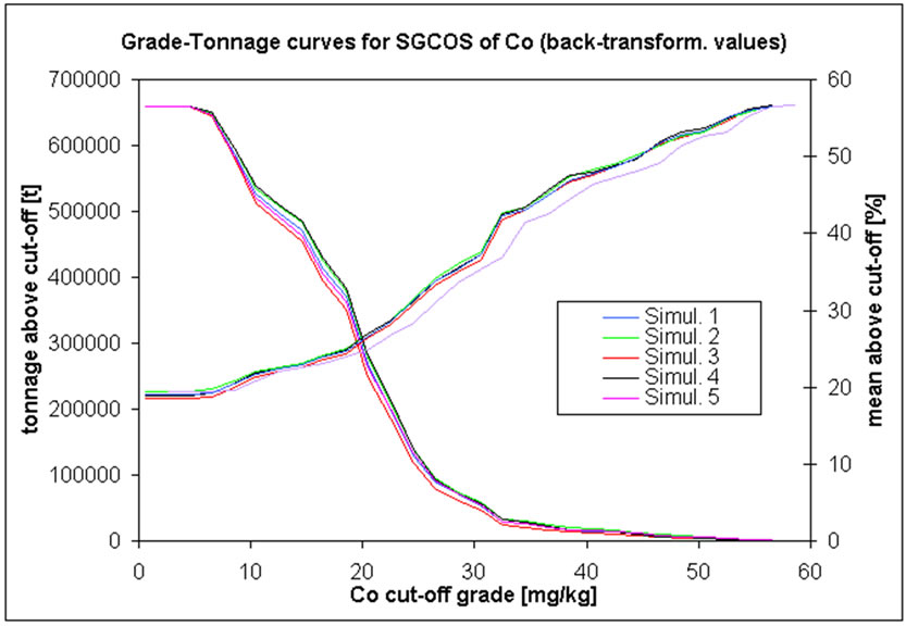 (b)
(b)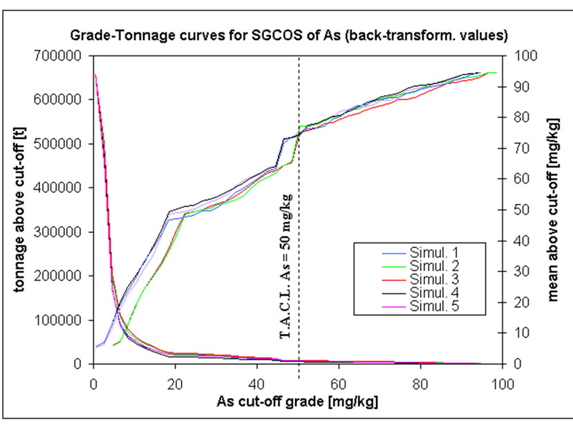 (c)
(c) (d)
(d)
Figure 14. G-T curves for five different SGCOS of: (a) Cr; (b) Co; (c) As; (d) Pb.
The main issues in this project were related to the nature of the data set. The boreholes are on an irregular sampling grid and there are very few samples in each borehole. Moreover, the lengths of the boreholes vary from 5 m to 20 m, the lengths of cores vary from 0.1m to 1.0 m) and sampling within a borehole is often discontinuous. The usual approach is to recomposite the samples to approximately the same length but the discontinuous nature of much of the sampling made this difficult.
The systematic nature of this discontinuous, smallscale sampling towards the bottom of the wells at, more or less, the same depth, indicates a logical reason for sampling in this way. In most applications the choice of a significantly smaller sample size indicates a significant increase in the variability of the variable being measured, which in turn implies an increase in the mean value of the variable (a proportional effect is present). This interpretation is borne out by the nickel grades for which there is a significant increase in the mean grade of the small (10 - 20 cm) samples collected at depths below 7.4 m. The mean grades of all other variables measured in these small-scale samples below 7.4 m are, however, lower than the mean grades of samples above 7.4 m. There are at least two possible reasons that could be advanced for the small scale sampling. The simpler, operational, reason is budgetary restrictions. This seems unlikely because the holes were sampled at different times and the small-scale samples are always below the 7.4 m deep. The more complex, and more interesting, reason relates directly to the variable (s) and the geology of the subsurface. There may be a change in structure, or simply a change in porosity and/or permeability at, or around, 7.4 m that causes some of the pollutants (in particular, nickel) to accumulate in small intervals. Alternatively, there may be a natural nickel anomaly below a depth of 7.4 m. Whilst the reasons for this small-scale, discontinuous sampling are, at present, unknown, the nickel grades of the samples are significant and must be included in the study.
Finally, it would be advisable to perform further sampling based on the simulation results obtained. The sparse data, especially in the vertical direction, affected the results of the simulations, in particular for the correlation correction simulations. More continuous and denser sampling undertaken in a few new boreholes could significantly improve the simulation results.
6. Acknowledgements
Enrico Guastaldi is indebted to Professors P. A. Dowd and C. Xu now at University of Adealaide, for admitting him to the MSc course at the Department of Mining and Mineral Engineering, University of Leeds in 2003-2004, and for their valuable explanations and suggestions about both geostatistics theory and this project.
REFERENCES
- P. A. Dowd, “Risk in Mineral Projects: Analysis, Perception and Management” Transactions of the Institution of Mining and Metallurgy (Section A: Min. industry), Vol. 106, 1997, pp. A9-A18.
- T. M. Burgess and R. Webster, “Optimal Interpolation and Isarithmic Mapping of Soil Properties. I. The Variogram and Punctual Kriging,” Journal of Soil Sciences, Vol. 31, No. 2, 1980a, pp. 315-331. doi:10.1111/j.1365-2389.1980.tb02084.x
- T. M. Burgess and R. Webster, “Optimal Interpolation and Isarithmic Mapping of Soil Properties. II. Block Kriging,” Journal of Soil Sciences, Vol. 31, No. 2, 1980b, pp. 333- 341. doi:10.1111/j.1365-2389.1980.tb02085.x
- T. M. Burgess and R. Webster, “Optimal Interpolation and Isarithmic Mapping of Soil Properties. III. Changing Drift and Universal Kriging,” Journal of Soil Sciences, Vol. 31, No. 3, 1980c, pp. 505-524.
- T. M. Burgess, R. Webster and A. B. McBratney, “Optimal Interpolation and Isarithmic Mapping of Soil Properties. VI. Sampling Strategy,” Journal of Soil Sciences, Vol. 32, No. 4, 1981, pp. 643-659.
- P. Goovaerts, “Geostatistical Tools for Characterizeing the Spatial Variability of Microbiological and PhysicoChemical Soil Properties,” Journal of Biological Chemistry, Vol, 27, No. 4, 1998, pp. 315-334. doi:10.1007/s003740050439
- G. B. M. Heuvelink, “Error Propagation in Environmental Modeling with GIS,” Taylor and Francis, London, 1998.
- P. Goovaerts, “Geostatistical Modelling of Uncertainty in Soil Science,” Geoderma, Vol, 103, No. 1-2, 2001, pp. 3- 26. doi:10.1016/S0016-7061(01)00067-2
- P. Goovaerts, G. Avruskin, J. Meliker, M. Slotnick, G. Jacquez and J. Nriagu, “Modeling Uncertainty about Pollutant Concentration and Human Exposure using Geostatistics and a Space-Time Information System: Application to Arsenic in Groundwater of Southeast Michigan,” Proceedings of the 6th International Symposium on Spatial Accuracy Assessment in Natural Resources and Environmental Sciences, Portland, Maine, 28 June-1 July 2004.
- P. A. Dowd and C. Xu, “GeostatWinTM—User’s Manual,” University of Leeds, Leeds, 2004.
- Gc. Bortolami, G. Crema, R. Malaroda, F. Petrucci, R. Sacchi, C. Sturani and S. Venzo, “Carta Geologica d’Italia, Foglio 56,” 2nd Edition, Servizio Geologico Italiano (Italian Geological Survey), Roma, Torino, 1969.
- G. Braga, E. Carabelli, A. Cerro, A. Colombetti, S. D’ Offizi, F. Francavilla, G. Gasperi, M. Pellegrini, M. Zauli and G. M. Zuppi, “Indagini Idrogeologiche Nella Pianura Padana: Le aree del Piemonte (P01-P02) e della Lombardia (Viadana e San Benedetto Po),” ENEL, Torino, 1988.
- C. W. Fetter, “Applied Hydrology,” 3rd Edition, Prentice Hall, Upper Saddle River, New Jersey, 1994.
- M.A.T.T. Ministero dell’Ambiente e Tutela del Territorio, Repubblica Italiana, “Environmental Minister Law DM471: Rules on Criteria, Procedures and Way for Environmental Remediation of Contaminated Sites,” 5th February 1997, Ordinary Supplement to Official Gazette of Republic of Italy, Rome, No. 293, 15 December 1999.
- F. Owen and R. Jones, “Statistics,” Pitman Publishing, London, 1994, p. 529.
- P. A. Dowd, “MINE5280: Non-Linear Geostatistics. MSc in Mineral Resource and Environmental Geostatistics,” University of Leeds, Leeds. 1996, p. 170.
- P. Goovaerts, “Geostatistics for Natural Resources Evaluation. Applied Geostatistics Series,” Oxford University Press, Oxford, New York, Vol. 14, 1997, p. 483.
- G. Matheron, “Les Variables Régionalisées et leur estimation: Une Application de la Théorie des Fonctions Aléatoires aux Sciences de la Nature,” Masson, Paris, 1965.
- A. G. Journel and C. J. Huijbregts, “Mining Geostatistics,” Academic Press Inc., London, 1978, p. 600.,
- J. P. Chiles and P. Delfiner, “Geostatistics: Modeling Spatial Uncertainty,” Wiley, New York, Chichester, 1999.
- H. Wackernagel, “Multivariate Geostatistics: An Introduction with Applications,” Springer, Berlin, 2003.
- R. Webster and M. A. Oliver, “Geostatistics for EnvironMental Scientists (Statistics in Practice),” John Wiley & Sons, New York, 2001.
- C. Lantuejoul, “Geostatistical Simulation: Models and Algorithms,” Springer Verlag, Berlin, 2002, p. 256.
- P. J. Ravenscroft, “Conditional Simulation for Mining: Practical Implementation in an Industrial Environment,” In: M. Armstrong and P. A. Dowd, Eds., Geostatistical Simulations, Kluwer Academic Publishers, Dordrecht, 1994, pp. 79-87.
- A. G. Journel and F. Alabert, “Non-Gaussian Data Expansion in the Earth Sciences,” Terra Nova, Vol. 1, No. 2, 1989, pp. 123-134. doi:10.1111/j.1365-3121.1989.tb00344.x
- C. J. Bleines, F. Deraisme, N. Geffory, S. Jeannee, F. Perseval, D. Rambert, O. Renard, Torres and Y. Touffait, “Isatis Software Manual,” Geovariances & Ecole des Mines De Paris, Paris, 2004.
- R. Dimitrakopoulos and M. B. Fonseca, “Assessing Risk in Grade-Tonnage Curves in a Complex Copper Deposit, Northern Brazil, Based on an Efficient Joint Simulation of Multiple Correlated Variables,” Application of Computers and Operations Research in the Minerals Industries, South African Institute of Mining and Metallurgy, 2003.
- I. Clark and W. V. Harper, “Practical Geostatistics,” Ecosse North America Llc., Columbus, Ohio, Vol. 1, 2000, p. 342.