Journal of Software Engineering and Applications
Vol.09 No.01(2016), Article ID:63064,43 pages
10.4236/jsea.2016.91001
Fault Handling in PLC-Based Industry 4.0 Automated Production Systems as a Basis for Restart and Self-Configuration and Its Evaluation
Birgit Vogel-Heuser, Susanne Rösch, Juliane Fischer, Thomas Simon, Sebastian Ulewicz, Jens Folmer
Institute of Automation and Information Systems, Technische Universität München, Munich, Germany

Copyright © 2016 by authors and Scientific Research Publishing Inc.
This work is licensed under the Creative Commons Attribution International License (CC BY).
http://creativecommons.org/licenses/by/4.0/


Received 13 December 2015; accepted 24 January 2016; published 27 January 2016
ABSTRACT
Industry 4.0 and Cyber Physical Production Systems (CPPS) are often discussed and partially already sold. One important feature of CPPS is fault tolerance and as a consequence self-configura- tion and restart to increase Overall Equipment Effectiveness. To understand this challenge at first the state of the art of fault handling in industrial automated production systems (aPS) is discussed as a result of a case study analysis in eight companies developing aPS. In the next step, metrics to evaluate the concept of self-configuration and restart for aPS focusing on real-time capabilities, fault coverage and effort to increase fault coverage are proposed. Finally, two different lab size case studies prove the applicability of the concepts of self-configuration, restart and the proposed metrics.
Keywords:
Industry 4.0, Automated Production System, OEE, Metrics, Recovery, Restart, Fault Handling

1. Introduction
In the course of Industry 4.0, intelligent products and production units are implemented. This includes production units with inherent capabilities which adapt (also structurally) flexibly in response to changing product requirements [1] or in case of failures of a partial component in order to stay or become operable again and increase the Overall Equipment Effectiveness (OEE) [1] . How can the adaptability, i.e. reconfiguration and restart of these automated production systems be evaluated and are these strategies already implemented in industry or is there still a huge gap to be bridged?
In the reference architecture (RAMI [2] ), attributes and requirements to Industry 4.0 components are specified and allow the evaluation of different solutions offered under the heading of Industry 4.0, but also serve for further development of attributes and metrics. In the following, one aspect of these requirements, namely adaptivity and selected metrics for adaptivity, particularly in the event of a fault, are presented to allow a comparison of different adaptivity concepts. Despite adaptivity already being discussed in academia, industrial automated production systems (aPS) lack such a concept. In systems design, consistency of models from different disciplines for specific purposes (fault analysis, safety) is required, but needs further analysis and support in the future [3] . To elaborate the challenge to realize such concepts in real world industrial applications, the state of the art in fault handling and software architecture as a basis for adaptivity after a fault is given, derived from eight industrial case studies (cp. Section 3).
The remainder of this paper is structured as follows. At first, the state of the art in engineering and operation of Programmable Logic Controller (PLC)-based aPS is given highlighting challenges and weaknesses in engineering processes, platforms and languages, domain specific extra functional challenges, concepts for recovery in case of faults as well as metrics to measure fault-recovery as a prerequisite for adaptivity. Next, an analysis based on eight case studies has been conducted to capture real world software architecture including concepts for fault-handling. Fault handling is chosen as it is strongly related to modes of operation in aPS and differs significantly from classical software also in embedded systems.
In aPS, operator personnel often has to fix faulty situations manually because the possible faults and fault combinations are manifold [3] and often need manual mechanical intervention by an operator.
The case studies reveal a software architecture with five levels of hierarchy with mostly hierarchical fault handling mechanisms on the one hand, but a lack of any automatic fault recovery as a prerequisite for adaptivity on the other hand. Instead, fault handling requires human intervention, therefore faults detected by the PLC need to be addressed in the human machine interface (HMI). We identified three different interface concepts in the case studies between PLC fault handling and HMI.
Despite the lack in realization in industrial aPS up to now, adaptivity concepts have been developed in academia and implemented in lab-size demonstrators for Industry 4.0, e.g. myJoghurt. To evaluate these concepts comparatively and measure the needed additional modelling or programming effort and the required real time behavior, selected metrics are introduced (in Section 4). Four different adaptivity concepts are applied and evaluated to lab size demonstrators in Section 5. The evaluation section closes with a comparison of the metrics’ results interpreting the significance of the metrics values in comparison. In Section 6, the summary and outlook for future development are given.
2. State of the Art―Challenges and Weaknesses
This section starts with an overview on the state of the art regarding model-driven engineering, platforms and programming languages for aPS, introducing modes of operation and finally alarm handling.
2.1. Development of Runtime Environments and Their Domain Specific Challenges of Programming Languages for aPS
After a short introduction to the specific characteristics of Programmable Logic Controllers, which are the standard industrial platform, and IEC 61131-3, which is the current programming standard, actual architectural approaches are introduced. Subsequently, the various challenges of developing software for aPS and challenges in the domain of aPS are described for a better understanding of maintenance issues of PLC code.
A. Platform, programming languages and software architecture in the aPS domain
Programmable Logic Controllers (PLC) are characterized by their cyclic data processing behavior, which can be divided into four steps. At the beginning of a cycle, the PLC reads the input values of the technical process, which are provided by sensors, and stores them in a process image. Subsequently, the PLC program is executed with the stored values and afterwards the output values are written, which control the actuators that influence the technical process. At last, the PLC waits until the cyclic time has elapsed. In a worst case scenario, if a fault occurs right after the input values have been read, the reaction time of the PLC is two times the cycle time.
The IEC 61131-3 programming standard for PLCs consists of two textual languages―Structured Text (ST) and Instruction List (IL)―and three graphical languages―Ladder Diagram (LD), Function Block Diagram (FBD), and Sequential Function Chart (SFC). Furthermore, the standard defines three types of program organization units (POU) to structure PLC code and to enable reuse: programs (PRGs), function blocks (FBs) and functions (FCs). The main differences between these POUs are that in contrast to FCs, PRGs and FBs possess internal memory and that FBs can be instantiated. Tasks are used to define entry points (PRGs) into a plant’s code, which are invoked depending on the defined cycle time of the task. The entry points (PRGs) then call other POUs which can execute code and sub-calls of further POUs. A regular PLC execution cycle consists of reading all inputs (sensors), triggering tasks depending on their cycle time and therefore their associated code (POU calls and subcalls), and finally writing all output variables (actuators). These cycles adhere to real time requirements, meaning that the defined cycle times of the tasks may never be exceeded.
Software engineering for aPS is still struggling with modularity, guidelines for appropriate software component sizes [4] - [6] and good practices for interfaces between these components. Katzke et al. [7] and Jazdi et al. [4] found different component sizes in aPS software (called granularity) and described the challenge to choose the best size and interface in between components for reuse and evolution. Cross component functions such as fault handling and modes of operation (manual, automatic) make the implementation of many modularity concepts difficult, which will be discussed in more detail in Section 3. Because in the plant manufacturing industry software engineering has been mostly project driven for decades, the challenge is to restructure legacy code from different projects with similar or even equal functionality. To make things worse, the different platforms (cp. Table 1) require software variants for the same functionality due to different IEC 61131-3 dialects.
Based on Katzke [7] the authors proposed a five level architectural model in [8] (cp. Figure 1). “A plant module resembles a whole production plant and, consequently, exists mostly in the plant manufacturing industry, but not in machine manufacturing industry. A plant module usually contains several facility modules, which re- present machines or plant parts such as a press or a storage system. Each facility module in turn consists of one or more application modules, which are machine parts that might be reused in other machines such as the material feed of a machine or the filling unit of a machine. Application modules are composed of basic modules which represent for example individual drives or sensors. Atomic basic modules represent the most fine-grained architectural level and refer to basic modules that cannot be decomposed into further module. The architectural levels can be used recursively, i.e., each level can consist of all module types of the more fine-grained levels.” [8] .
Vyatkin proposes a software architecture for distributed automation systems based on IEC 61499 [9] [10] . The resulting software shows a composite structure and consists of event-driven FBs, which are used to describe processes. Although first industrial applications confirm the standard’s benefits, e.g., reduced time and effort to develop automation software, a high degree of code modularity and a high potential for reuse, the standard is not commonly used within industry at present.
Current research in the field of model-driven engineering (MDE) is mainly focused on developing new methods to support the development process of new software using modeling languages such as UML or SysML. Unfortunately, there is a big gap between existing legacy code on field level, i.e. PLC code, and the vision and

Figure 1. Architectural layers from [8] .

Table 1. Table classified case studies based on and enlarged from [8] .
PT―process technology, MT―manufacturing technology, P―plant, PU―plant unit, M―machine, Eng―Engineers, Tec―Technicians, S―Skilled Workers, na―not available, (O)―partially realized.
attempt to introduce an MDE approach in industrial companies supporting a systematic maintenance and software evolution. To bridge this gap, at first code refactoring and building of appropriate software components is required. Bonfè et al. introduce the concept of mechatronic objects to enhance modularity of the software, which can be represented in control programs by FBs. While the structure of the aPS is modeled using UML class diagrams, the behavior can be defined with UML state diagrams [11] . Although various models for software architecture have been developed, accepted software architectures are missing in aPS up to now.
B. Constraints due to size
While machine manufacturers are able to commission and test their products before delivering it to the customer, plant manufacturers are unable to commission the entire plant in their own facilities due to the weight and the size of the components. A press for example is too large to be transported fully assembled on a ship and thus needs to be transported in smaller pieces and be assembled afterwards at the customer’s site. Consequently, commissioning and startup of complete plants is done on site with the customer pressing to start production, which leads to high time pressure. Furthermore, it is common that the start-up staff on site includes only technicians or skilled workers instead of the application engineers who developed the PLC software for the plant. Therefore, the communication between development engineers in the office and technicians on site needs to be coordinated which can be challenging in a company that distributes its products globally due to different time zones and time pressure with high penalties.
C. Extra functionality challenges: modes of operation and fault handling
In addition to implementing the control functions that are carried out by an aPS, also aspects like different operation modes or visualization must be taken into account.
According to Güttel et al. [12] the main operations of function blocks include:
Automatic mode: defines the behavior of a machine part in automatic mode.
Setup mode: defines the behavior of a machine part in setup mode. In this mode, the drive of a machine part moves as long as the manual input is active. In this mode, no interlocks are active.
Manual mode: defines the behavior in manual mode. In this mode, the interlocks are active.
Semi-automatic mode: defines the behavior of a machine part in semi-automatic mode.
Initialize: defines the behavior during the initialization of the machine part.
Shut down: defines the behavior during shutdown.
Save stop: defines the actions which are necessary to reach a safe state.
The different operation modes need to be implemented, which may be realized as additional automata or different branches with the other automata according to Fantuzzi et al. [13] . In food & beverage a more sophisticated standard is used, i.e. the OMAC standard or in Germany the Weihenstephan Standard [14] .
The OMAC State Machine [15] (cp. Figure 2) is part of the widespread PackML standard, which pursues the objective to bring operational consistency to a packaging line, especially if it consists of packaging machines from different vendors. The PackML standard defines the OMAC State machine with 17 states consisting of acting and waiting states in which acting states represent activities like starting and waiting states identify the reaching of a set of conditions e.g. Held. The OMAC State Machine is responsible for identifying valid state transitions depending on the actual OMAC state and specified state transition conditions. If a state change occurs, a suitable function is called, that is implemented by the machine vendor or integrator.
2.2. Fault Recovery and Restartability in aPS
In the following four different concepts for fault recovery to increase OEE by adaptation are introduced in principal. Fault recovery after a device fault may be realized automatically in case of redundant information/devices available. The redundant information may originate from an additional device and a Fault Coverage Analysis (cp. Section 5.1 according to [16] ) providing the faulty information or from a redundancy model designed pre- runtime and calculated during runtime using other process information (cp. Section 5.3, [17] ). Both scenarios will be discussed and evaluated with the metrics to be introduced during the evaluation examples. The third scenario focuses on restart after emergency shutdown remembering the position of the work piece to restart properly, which is modelled accordingly during the design phase (cp. Section 5.3). The fourth scenario examines restartability after machine stop [18] to ease the operator’s task and reduce operator interaction. This approach is based on an OMAC State Machine (cp. Section 5.4).
Concerning the elimination of faults our work is based on prior results by Schütz et al. [17] about dynamic reconfiguration and, if present, an indirect replacement sensor being used to substitute a defect sensor or actua-

Figure 2. OMAC state machine including waiting states (dashed-dotted framing), acting states (dashed framing) and the dual state execute, which is both a waiting and an acting state (bold framing).
tor with a virtual sensor, but with less accuracy. Schütz et al. [19] have developed a model-based approach for this based on SysML and are able to automatically generate executable PLC-code for the knowledge base from this model. Priego et al. developed an architecture that allows the definition, generation and update of a PLC’s software architecture during runtime in response to modeled changes on the plant layout, the product to be manufactured or the control hardware. [20] . Andersson et al. [21] [22] address the challenge to automatically derive operation sequences for restarting manufacturing systems (and here especially assembly cells typically used in the automotive industry). In context of these works, restarting is the procedure to “resynchronize the control system and the physical system, such that the production can be restarted and eventually complete” [23] . These concepts are required because the intended nominal production is not performed due to an error during operation. The concept is based upon the concept of self-contained operations which contain information about their potential sequential relations to other operations and, accordingly, can be arranged to so-called sequences of operations [24] . For modeling possible operation sequences, Andersson et al. rely on extended, deterministic, finite automata and supervisory control theory formalisms (i.e. controller synthesis) for deriving a desired restart strategy. Nevertheless, flexible manufacturing systems facilitate the production according to multiple operation sequences [25] . Therefore, Bengtsson et al. [26] [27] extended the modeling concept to multiple operation sequences. Here, identification of an earlier state to restart the system is more complex and requires efficient algorithms. Based on this approach, Bergagård et al. [18] [25] generalize the approach for restartability of Andersson et al. by extending the concept to multiple resources to be restarted (i.e. multiple operation sequences). This broadens on the one hand the set of manufacturing systems which can be addressed by this approach and on the other hand, by means of the generalization, also more efficient synthesis algorithms can be applied [23] .
2.3. Metrics for Adaptive aPS
As characteristics for Quality of Service real-time capability, reliability and the possession of the required QoS- attributes are named in RAMI. If solely the Overall Equipment Effectiveness (OEE) is used as metric for reconfiguration during runtime in case of failure, statements on the continuity of production despite a fault and the following possible output and its quality can be made. In the following already existing metrics for flexibility and adaptivity are summarized as a basis for the derivation and presentation of the developed metrics presented in this paper. Ladiges et al. [28] present metrics for flexibility divided into machine flexibility, process flexibility, routing flexibility and operation flexibility for discrete production processes. Thereby, the absolute machine flexibility is defined as number of operations that can be performed without any form of manual intervention. In contrast to that, Ladiges et al. [28] calculate the relative machine flexibility as a machine’s number of operations without manual intervention, which can be performed in reference to all tasks within the facility, for example, tasks which can be taken on by other machines. Gronau et al. [29] establish an evaluation scheme for adaptivity within the scope of business-specific versatility and distinguish between five levels: no adaptation possible, adaptable via add-ons, adaptable via modification, adaptable via parameterization and adaptability via self-con- figuration. In the following we focus on adaptability via self-configuration in case of faults. Wiendahl et al. [30] define characteristic features for reconfigurable production and assembly systems e.g. modularity and scalability. Raibulet et al. [31] present several metrics for adaptivity from the perspective of computer science, classified according to architecture metrics, structural metrics, performance metrics and interaction metrics. Thereby, the main focus of architectural metrics lies on the costs of adaptivity. Structural metrics emphasize code changes due to the adaptivity and thus the additional required code entities while performance metrics rate the response delay caused by the adaptations as well as the response quality. The latter aspect is, in the following, adapted for production automation, formulated and evaluated. Regarding interaction Raibulet et al. [31] distinguish between users, which are operators in our case, maintenance personnel and administrative interaction (engineering).
3. Results of the Case Study Analysis on Fault Handling and Software Architectures within Industrial Automation Software for aPS
In industrial practice in machine and plant engineering, initially the general software architecture and especially handling of faults was analyzed in order to examine how reconfiguration and recovery in case of faults is already or will be implemented in future and which challenges thereby arise and finally how to evaluate different strategies with metrics.
In cooperation with eight different companies in the field of machine-and plant engineering, ranging from special purpose machine manufacturers (Case studies A, B, E and H) to plant manufacturing industry (Case studies C, D, F and G) (cp. Table 1 for an overview of the case studies), a five-staged architecture model has been confirmed (cp. Figure 1) and, exemplary, the fault handling mechanisms were assigned to these five levels in order to analyze differences and similarities regarding fault handling and its integration into the software architecture (cp. Figure 3). Hereafter the characteristics are shortly introduced.

Figure 3. Fault handling in the case studies sorted into the five levels of the control software architecture (enlarged from [8] ).
The case studies differ regarding the constraints due to size (row number of components, number of supplier’s library components, and size of memory), i.e. delivering machine units or entire plants. Especially in plant manufacturing different platforms, i.e. PLC types need to be supported due to worldwide customers’ requirements and as Vogel-Heuser et al. [3] already discussed on-site changes even by less qualified customer staff are mandatory to reduce downtime (row maintenance staff), which mostly leads to the usage of very simple programming languages, i.e. IL and LD. In some industry sectors, e.g. food & beverage domain specific standards occur to support the interlinking of different machines to one plant, e.g. OMAC and Weihenstephan Standard delivering a joined understanding of machine states. Regarding fault recovery and restart there is still a lack in industrial software, which will be discussed in the following.
The eight investigated case studies all implement hierarchical fault handling strategies with special forms. Considering real-time metrics is simple: The cycle time for fault detection amounts to one cycle. Isolating the fault may take several cycles if, for example, the group error has to be analyzed first. Rather than making the expense of fault isolation, which is occasionally fairly high (especially in case of alarm showers), the operator is provided with all alarms and following alarms connected to the fault. However, in order to carry out suggested reconfiguration and self-healing measures fault isolation is mandatory. Software-based, virtual sensors are so far not implemented in any of the industrial case studies, so that reconfiguration of functions via soft sensors, i.e. self-configuration according to Wiendahl [30] is not possible. In the following for four of the eight case studies fault handling is discussed in more detail to provide a deeper understanding of the domain.
Case study A―Special Purpose Machinery in Factory Automation for Automotive Sub-Component.
The first case study was conducted in the area of factory automation for production of automotive sub-com- ponents. In this domain, machinery is designed to customer’s order (special purpose machinery) and thus the company has created a software structure which standardizes the software hierarchy within each unique machine. The structure is oriented at the hardware modules which are as follows: A production line (plant module) consists of multiple facility modules (each controlled by one PLC), which in turn consist of multiple application modules (larger sub-modules within the facility module, often representing one production process step). The structure definition allows for further subdivision of application modules into smaller application modules if reasonable. The most basic modules represent standard and special components such as pneumatic cylinders or vision systems.
The program of a facility module is usually limited to one task, which invokes the program block representing the program entry point. General program parts relating to the facility module and program parts relating to individual application modules of the facility are invoked from this entry point. The general program parts repre- sent functions such as diagnosis or initialization functions for the hardware controlled by this particular PLC. The entry point for each application module is a managing program block (program block related to decisions about sub-calls rather than direct relation to functionality of the application module), which is used to trigger sequences depending on the operation mode and initialization status. Invocation of further hierarchy layers using the same pattern can also be realized in the managing program block. Both general program parts and application module related structures invoke library functions, e.g., for communication to standard or special components.
Fault and alarm handling and subsequent error handling is initiated by atomic, basic or application modules. Atomic and basic modules include diagnosis functions for the connected modules, allowing simple fault detection, such as for stuck cylinders. Application module fault handling deals with errors in the process sequence which can result from failures of basic modules or the process itself. In addition, the application modules’ managing program block monitors safety functions, such as safety door switches. Whenever a fault is detected, an alarm is collected in a centralized array alongside the facility module layer (cp. Figure 3, path A) and displayed on the HMI (cp. Figure 5, Fault Handling I). In case this fault is detected by a basic module, information directly relating to the component ID is included in the error message (cp. Figure 5, Fault Handling III). At the same time, the respective module changes into an error state and passes on the information to the parent module (cp. Figure 3, path B). This module in turn can implement failure handling algorithms, which are triggered according to the alarm. At the same time, the application modules’ managing program block monitors status variables collected in the status structure and can halt automatic sequences in case of serious errors. In contrast to the concepts of some of the other case studies, the hierarchical module structure is partially bypassed by the centralized fault recording and status structure.
The machine state is realized through the operation modes and is loosely comparable with the OMAC states “execute”, “aborting”, “aborted”, “resetting” and “starting”. In automatic mode, the module is executed and aborted in case of errors resulting in a failure state (“aborted”) which requires human interaction. The resetting is done by switching to manual mode, used to resolve process errors, followed by an automatic recalibration of the machine (“starting”), which is a prerequisite for returning back to automatic mode. Besides the facility module, each application module possesses these different operation modes, allowing for sub-states in the machine. While the OMAC state machine is not used, this procedure of switching between machine operation modes and thus states is standardized within this company.
Case study B―Machinery for Packaging Industry
The example in case study B consists of three tasks which invoke three PRGs. The task with the second highest priority and its corresponding program realize and call the main functions controlling the technical process and are strongly related to the mechanical layout of the machine. The mechanical layout consists of one facility module and six main application modules, which is directly reflected within the PLC control software architecture (with the exception of several additional software modules being used for facility-wide functions, e.g., for error management). Each application module includes similar subroutines, such as parameterization or axis movement, which are implemented differently and mostly include additional application and basic modules. Furthermore, encapsulated FBs and functions are used which stem from a supplier delivering and supporting axes in particular. The application conforms mostly to the ISA-S88 and implements the OMAC state machine model.
Fault and alarm handling may be considered as being handled in a hierarchical manner (cp. Figure 3). On the basic module level the main part of fault/error detection of hardware and faults stemming from the technical process is happening. This is only logical as, e.g., a pneumatic cylinder not reaching its end position, should be identified by the basic module pneumatic cylinder. It allows for easier reuse, as the mechanical representation has a direct software implementation. However, the error ID is assigned on the next higher level along with the decision on how the identified error should be handled (related to the severity of the error in rising order: only a warning is issued, the machine is immediately shut down). The advantage in this kind of setup is that errors are assigned to the correct application module (e.g., which pneumatic cylinder in which module is erroneous), making error identification easier. Furthermore, if more than one error occurs within one application module, but from different basic or sub-application modules, an analysis can be done and group errors, hinting more specifically at the cause of an error, may be identified. Group errors lead, depending on their severity, to the shutdown of the entire machine group as they often hint at specific problems in the specified group (area of a machine). In the next step the errors are analyzed by separate functions, apart from the application modules when considering the mechanical layout. The functions collect all errors and implement the error reaction. If several errors arrive, which individually would only be reported, the error reaction of shutting down may for example be set. This kind of setup allows for easy maintenance, as the overall error management functions have been standardized as libraries and can be reused within every machine. The error detection and error reactions are carried out mainly within the second task. The task with the lower priority executes functions related to the HMI (sending the alarms).
After an error that leads to a shutdown has occurred a function for restarting is available. If the calibration has not been impaired by the shutdown and the material is not entangled somewhere in the machine, the operator can decide to acknowledge the error and restart using the implemented function.
Case study D―Plant Manufacturer: logistics process
The storage system analyzed in case study D consists of five application modules (for a detailed description cp. [32] ) and alarm handling within the storage is divided according to these five modules. Within the application module “general functions” a few general storage alarms, i.e., safety door alarms, are generated and also alarms of other application modules, such as “storage car” or “interface functions”, are collected. If more than one storage car is used in the storage system, the application module “storage car” is reused and the alarms of the second car are also used for interlocking conditions in the first car’s application module and vice versa. Depending on the severity of a detected fault (for example failure in application module “storage car 1”), the whole facility module “storage” or only parts of the storage system (storage car 1 stopped, but storage car 2 still operating normally) is switched to emergency mode. The shutdown of single application modules (e.g., “storage car 1”) or the entire facility module “storage” according to the severity of the detected error is similar to the group errors described in case study B. If the facility module storage system is switched to emergency mode, the alarm is, additionally, collected on plant module level. After a delay time, the preceding facility modules, which transport production goods to the storage system, need to be stopped as well, due to a limited buffer for accumulated production goods. In summary, alarm handling in case study D is implemented in a hierarchical manner (cp. Figure 3).
Case study E―(Special) machinery in packaging
In this case study, a well-defined software architecture is used that corresponds mainly to the physical layout of the machine. The latter is divided in several modules on application level which are all initialized and controlled by a facility wide module control (cp. Figure 4). Each module has again one or more submodules and each submodule uses one or more basic elements. Furthermore, every module has got its own and independent state machine according to the OMAC standard [15] and passes on its state to its belonging submodules which―just like the modules―execute routines according to the given state. In these routines corresponding commands are given to the belonging basic elements. Additionally, the supervisory module control has got an own state machines well and is able to cause state switches of the modules by a defined set of commands via the respective interfaces.
Such a state switch can be induced by an occurring error, e.g. in a submodule, which is reported to a facility wide diagnostic module. The latter evaluates all reported errors and as a result sets an according diagnostic mode. Additionally, the module in which the error occurred immediately switches to the state aborting. Depending on the severity of the error, all other modules may have to be either stopped or aborted which is taken into account by the diagnostic module. Depending on the diagnostic mode, the module control subsequently sets a respective command to force all other modules to switch to the state stopping or aborting respectively. Hence, all modules have independent state machines but they are coordinated by the commands of the facility wide module control.
There is no full restart function available after the machine has been shutdown due to an error. However, axes that have been interrupted in their movement automatically move into a respective position from where a restart is possible.
After a more detailed analysis of the four case studies regarding fault handling discussing the concepts of restart and self-configuration in all cases, we can summarize that due to the character of the technical process and

Figure 4. Software architecture and fault handling―case study E (figure caption).
the resulting plants, implementing restart functions is not always possible. Since some plants (such as case study D, F, G) contain continuous as well as discrete processes, a high number of interventions and different states arise and especially the continuous processes are highly interconnected. Furthermore, material properties often change during a continuous process and it is therefore not possible to return a plant into a previous recovery state with a defined material property, since once changed, an earlier material property cannot be retained.
Because of the missing restart and self-configuration abilities in industrial case studies, operators need to readjust the machines and plants into an appropriate state by manual intervention and via HMI interfaces. As interface to the operator three main variants to handle fault detection and fault handling with HMI (Human-Machine-Interaction) were identified (cp. Figure 5).
In variant I, faults are detected at the lowest level and collected in an array within a Function Block (FB Fault). Every fault that might occur in the machine has a unique, machine-wide fault ID. Furthermore, the entire machine is hierarchically divided into modules as depicted in Figure 5 with each of the modules and submodules having a unique identification and a unique instance number. After a fault is detected on submodule or module level, fault ID, module and submodule ID as well as module and submodule instance number are combined to form an unambiguous fault number, which is transferred to the Function Block FB Fault. By analyzing the final fault number, the fault type as well as its exact location within the machine can be determined. This approach to fault handling has, due to the unambiguous fault numbers, a high degree of flexibility (concerning, for example, the addition of further machine modules).
In contrast to variant I, the fault ID in variant II is not based on the occurring fault and the according fault location, but each component of the plant, such as an actuator (e.g. drive) has a determined address within a data block DB HMI to transfer the component’s alarms to. However, if the plant’s components need to be altered or changed, addresses cannot be changed. This leads to unused memory when removing a component (cp. Variant II in Figure 5: removal of Drive 2 leads to unused memory in DB HMI) and, moreover, the addition of a further component is only possible, if a spare address in the data block has been provided. Therefore, this fault handling approach has only a limited flexibility in regard to removing or adding plant components such as drives.

Figure 5. Identified variants of fault handling in between PLC and HMI interface as analyzed in the case studies.
In variant III, every plant component is assigned a unique component ID. This component ID is not only used in the software, but also in the plant’s construction plan or the circuit diagram and, therefore, supports working in an interdisciplinary development team. The software includes a data block for every actuator, which contains all variables belonging to this actuator (e.g. input and output variables or internal variables). Thereby the data blocks can be mapped to the according actuator by means of the component ID. Once a fault is detected on the lowest level (in an actuator), a variable in the according data block is set. The fault variables of each actuator are collected in a super ordinate status data block (cp. Figure 5, right: Status DB of a Conveying-Module including various drives and their component IDs) and the information in this status data block is transferred to the HMI including the component IDs. The flexibility of this fault handling approach is high due to the use of component IDs−unlike variant II the actuators are not assigned a specific address in the status data block, but can be identified based on the component ID. Furthermore, the component ID associated to a fault message serves to locate the fault within the plant.
4. Proposed Metrics for Adaptivity Focusing on Fault Handling
To ensure the quality of service of Industry 4.0 systems, it is essential to fulfill required real-time capabilities as well as adaptability, e.g. self-configuration as well as restart after a fault.
Therefore, in the following the performance metrics according to Raibulet et al. [31] are adapted for the field of automation with focus on fault detection in real-time, since the adaption in an event of fault during runtime is mandatory in order to render the required quality of service in this respect as well. In the following we regard real-time techniques, which are able to identify faults, isolate faults and introduce countermeasures during runtime.
Initially, metrics for the evaluation of real-time behavior during identification, isolation and elimination of faults are considered and, subsequently, selected metrics regarding the proportion of detectable faults in respect to potential faults are discussed under the heading of fault coverage. The proposed metrics to measure adaptivity of aPS are depicted in Figure 6.
4.1. Real-Time Capability
Programmable Logic Controllers (PLCs), which are used in manufacturing automation, operate cyclically.

Figure 6. Proposed metrics for adaptivity for aPS.
Therefore, the number of PLC-cycles for fault detection, fault isolation and fault reaction need to be observed. Fault isolation refers to the unambiguous allocation of a fault to its cause, for example a device.
In the following a measure for implemented faults in a machine or plant needs to be found, which displays the coverage of potential faults by an automatic reconfiguration in relation to all potential faults.
 (1)
(1)
An index for the survey of the punctuality of fault detection is the plcDFAI (PLC-cycles to detect faults adaptivity index, cp. Formula (1)). It is calculated by multiplying the number of cycles, which a PLC-implementation needs to detect a fault (pcycles), and the cycle time (tcycles), which is configured in the PLC. The result is an approximation of fault detection time based on the PLC cycle.
 (2)
(2)
As soon as a fault is detected, it has to be isolated, whereas here again the fault isolation is to be understood as unit-afflicted time. Analogous to plcDFAI, the plcIFAI (PLC-cycles isolate fault adaptivity index, cp. formula (1.2)) is calculated by multiplying the number of PLC-cycles needed for fault isolation (icycles) and the configured cycle time (tcycles).
 (3)
(3)
Once the fault is detected and isolated, strategies can be performed PLC-based in order to compensate the fault. Depending on the applied fault compensation strategy the number of PLC-cycles needed for fault compensation varies drastically. To conduct an assessment in case the method based on Schütz et al. [17] is used, the plcFCLAI (Plc-cycles for switching to software based sensor, cp. Formula (3)) is defined as the number of PLC-cycles needed to switch from real sensor to virtual sensor (ncycles) multiplied with the configured cycle time (tcycles).
 (4)
(4)
The sum of the time for fault detection, fault isolation and fault compensation results in the total time for fault handling, given in Formula (4).
4.2. Real-Time Capability
The development of fault models is frequently conducted with Fault Tree Analyses (FTA) [33] in order to be able to calculate the failure probability of functions and of the overall system based on basic events and their failure rates. The term fault coverage is especially used in the field of testing [34] . According to the fault classification by Friedrich et al. [34] we examine faults that are repairable without manual intervention.
In contrast to the standardized Fault Tree Analysis, in our approach basic events are used to display physical phenomena, which need to be made measurable in order to detect the faults modeled on a superordinate level. Therefore the new term Fault coverage analysis (FCA) is used. A hierarchy of these higher-level faults can be developed in accordance with DIN 25419 [33] .
By modeling the basic events the system developer is able to estimate the covered faults at an early stage of the plant’s life cycle by utilizing metrics. By comparing basic events which have already been made measurable by a plant expansion stage (with sensors), fault coverage can be calculated by using the BECAI (Basic Event Coverage Adaptivity Index, cp. Formula (5)).
 (5)
(5)
The BECAI corresponds to the number of basic events, which are covered by measurement-technology (c), divided by the total number of modeled basic events (b) and indicates the proportional degree of coverage ranging from 0 (0%) to 1 (100%)
Consequently, from the BECAI follows the proportion of basic events that are not covered by measurement-technology and are, therefore, not detectable. This index is called BENCAI (Basic Events Not Covered Adaptivity Index, cp. Formula (6)).
 (6)
(6)
The BENCAI directly results from the proportion of basic events not covered by the BECAI or as a result of dividing the summation of all basic events which are not covered (nc) by the total amount of basic events modeled in FCA (b).
The modeled basic events in level 1 of the FCA are directly linked to the faults on level 2 (see Figure 8). If all basic events that lead to a fault are measurable, then the fault is detectable. The FLCAI (Fault Level Coverage Adaptivity Index (cp. Formula (7)) describes this coverage.
 (7)
(7)
Formula (7) calculates the proportion of faults which can be covered on a level j in the FCA with regard to the total number of faults modeled on level j of the FCA. This procedure is applicable to all levels of the FCA that are above the basic event level, all the way up to the top-level node of the FCA. The result is the fault coverage on level j in percent.
4.3. Minimal Programming Effort to Increase Fault Coverage
The fault coverage formula in Formula (7) also indicates the number of uncovered faults. In order to examine, which fault may be detected with a minimal enhancement effort, the MEICAI (Minimal Effort to Increase Fault Coverage Adaptivity Index, Formula (8)) is defined.
 (8)
(8)
The MEICAI shows those faults i on FCA level j with the highest number of coverage of basic events covered (BEC) in proportion to basic events not covered (BENC). All faults on level j are included and the above-mentioned calculation is carried out, whereby the fault is chosen, which has the minimum aspect ratio of BENC to BEC and, therefore, contains few BENC but a maximum amount of BEC. Only faults with a number of BENCs higher than 0 are included in this calculation because otherwise the MEICAIj is 0 and, therefore, all basic events are already measurable and covered.
The MEICAIj indicates the fault that can be covered with minimum effort. In order to estimate the required effort further, for mechatronic systems changes of software and automation hardware as well as changes of the mechanics need to be considered. This article focuses on software changes.
In order to implement the identified fault detection and compensation strategies, with minimum effort for fault compensation in software, adaptations in the software is needed that have to be made in the languages of the IEC 61131-3 standard-in this example the language function block diagram is chosen. The internal behavior of the FBDs is thereby not considered (cp. Fuchs et al. [35] ).
For an estimation of the effort for the required software changes the FHAI (Fault Handling Adaptivity Index, cp. Formula (9)) is introduced.
 (9)
(9)
The FHAI calculates the proportion of newly added (FHAInew), adapted (FHAIadapted), removed (FHAIremoved) and unchanged (FHAIold) software elements of each function block in IEC 61131-3. If, for example, all software elements have been changed and, thus, no unchanged software elements remain, a proportionate effort of 1 (100%) needs to be summoned because FHAIold equals 0; whereas, if no changes are conducted, the FHAI is 0. Therefore, the FHAI gives the proportion of software changes, which need to be conducted in order to guarantee adaptivity, in percent.
The single factors of FHAI are defined as follows within (10) to (13).
 (10)
(10)
 (11)
(11)
 (12)
(12)
 (13)
(13)
For instance, FHAInew, Formula (10), is calculated by summarizing the sum of newly added inputs (inew) and newly added outputs of the function block (onew) and the sum of newly added function blocks itself (fbnew). The calculations for adapted (FHAIadapted), removed (FHAIremoved) and retained software elements (FHAIold) are carried out equivalently. Using IEC 61131-3 function block diagram, it may occur that the output of a function block is, at the same time, the input for one or several other function blocks. These interconnections are included in the FHAI calculations as inputs as well as outputs, since they either remain unchanged as inputs and outputs (oold) or they are changed (onew, oadapted and oremoved).
In this section the programming effort was measured. In Schütz et al. [19] the necessary code was generated from a model (SysML), therefore for an MDE based approach instead of a programming effort the effort to adapt the model should be evaluated. But nevertheless for the maintenance staff the additional programming effort is interesting as an indirect measure program comprehension according to Vogel-Heuser [36] .
4.4. Minimal Modeling Effort to Increase Fault Coverage
Frey and Litz [37] introduced complexity metrics for Petrinets using besides others an adapted McCabe metric. Chidamber and Kemerer developed a set of metrics of OO design [38] , e.g. weighted methods per class (WMC) which is a measure for class complexity used in this paper: in order to calculate the WMC of a program, the cyclomatic complexity measure of each method is summed up for all classes, cp. [39] . WMC and the cyclomatic complexity measure have already been successfully applied comparing task complexity for usability evaluation [36] . The cyclomatic complexity measure by McCabe [40] is calculated as stated in Formula (14),
 (14)
(14)
with e being the number of edges (like transitions in a state chart), n being the number of nodes (states of a state chart) and p being the number of connected components (number of analyzed state charts). The complexity measure V(G) represents the number of linearly independent paths through the analyzed graph.
In the case of model changes in UML or SysML state charts the McCabe metric is applied instead of the metrics introduced in Section 4.3, since the necessary changes of the state charts are restricted to adding or removing states and transitions.
As a metrics for the relative modelling effort FHAImodel:
 (15)
(15)
This mathematical comparison can also be used to compare the complexity of software evolutions, standardized by the mean value of compared software evolution. Due to the standardization, it is possible to compare pairwise different independent software evolutions, to point out an evolution, in which complexity does increase too much, e.g. to ease software maintenance.
Furthermore, three cases concerning FHAImodel can be stated shown in Formula (16). The first case indicating that the cyclomatic complexity measure of both models stages is equal. Hence, FHAImodel indicates no increasing or decreasing model complexity. Furthermore, as soon as the new model evolution has a bigger cyclomatic complexity, FHAImodel indicates it resulting in a positive number. The last case indicating a decreasing model complexity in case of the new cyclomatic complexity is less than the old cyclomatic complexity, resulting in a negative number.
 (16)
(16)
5. Evaluation of Defined Metrics by Means of Three Different Types of Adaptive Strategies Using Two Different Laboratory Demonstrators
In this section the metrics defined in the previous Section 4 are applied to different simple lab demonstrators: a pick and place unit plant (a) PPU (cp. Figure 7) as well as its extended version (b) (cp. Figure 16 in Section 5.4) (both demonstrators of the PP 1593 design for future-managed software evolution) and a tank of a process plant (c) (cp. Figure 14).
For all four scenarios the realized concept of adaptation is shortly discussed at first and thereafter the scenario is evaluated using the proposed metrics.
Using two different lab size demonstrators four different application examples representing different types of adaptivity are introduced in this section. The first and the third application scenario represent fault detection, fault isolation of a faulty device, e.g. a sensor and self-configuration to continue operation. The second and fourth represent strategies to restart after a malfunction, e.g. a stop or emergency shutdown. In the first application example sensor redundancy is given and on this basis the faults can be isolated (5.1) as a prerequisite for later restart. Self-configuration of a model based redundancy for a tank level in case of a sensor fault is discussed in Section 5.3. The second scenario stores the state of the machine in case of an emergency shut-down and remembers the position of the work piece to restart properly. The fourth application example uses the extended xPPU for a state based restart based on an OMAC state machine in case of faulty position of work piece and a resulting machine stop (5.4).

Figure 7. Converyor belt of the lab size application example Pick and Place Unit (PPU).
5.1. PPU-FCA Based Fault Detection and Self-Configuration with Redundant Sensor Device
In the sorting unit of the plant work pieces are distributed to three different slides (Sorting 1-3) according to their color and material. Each slide is equipped with an inductive sensor (sens_slide). Each pusher has a front and a rear end position sensor as well as an analogous sensor for precise position measurement. The analogue sensor represents the redundant sensor device to measure the position of the pusher. All malfunctions leading to the report of a timeout error and the malfunctions’ causes are considered (cp. Figure 8) and it is analyzed to what extent it is possible to automatically assign them.
In Figure 8, a fault tree with potential causes (basic events) and their logical contexts, those indicate a fault, are depicted. The fault tree itself only refers to the conveyor unit (cp. Figure 7) consisting of sensors for material detection in order to sort different kinds of work pieces in according slides. The light gray colors indicate causes, which can be detected with a basic configuration of the PPU via measurement technology. For instance, basic event p7 represents a binary sensor at the slide of the sorting unit, which detects the incoming material of a work piece.
To identify failures to be handled automatically, the FCA is used. The realization of self-configuration functionality presumes that failures have to be observable by the software (i.e. adequate sensors are installed to identify a specific failure) and automatic compensation mechanisms (analogously to maintenance instructions) have to be implemented. Therefore, the PPU’s self-configuration variant consists of additional sensors. For example, to detect a “WP Jam” within the sorting station, pushers previously consisting of binary positioning sensor are substituted by pushers equipped with analogue transducers to precisely detect the pusher’s positions (parameter sens_transducer in Figure 7). The installation of an additional pressure sensor facilitates the detection of pressure failures (cp. Figure 8, p. 1). Sensors are installed at each slide to detect arriving WPs by monitoring for rising edges of the sensor signal (sens_slide, cp. Figure 7).
In the following the metrics defined in Section 4 are applied to the PPU.
5.1.1. Metrics for Real-Time Capabilities
According to the definition in Section 4.1 various metrics for real-time have been defined. The metrics for real-time capabilities are applied to two software variants implemented in sequential function chart (SFC, defined in the IEC 61131-3 standard, cp. Figure 9). The variants are compared in order to determine (by means of the metrics) which one of the two implementations shows better real-time characteristics; thus, shorter cyclic times for plcFCLAI (cp. Formula (4)).
Fault detection, selection and compensation are performed simultaneously in three states (cp. Figure 9, left). In an IEC 61131-3-runtime environment simultaneous states are passed through within one cycle time. Thus, the plcFCLAI results to 30 ms, on the assumption that the PLC-cycle time is configured to 30 milliseconds.

Figure 8. Part of a FCA regarding time monitoring of work piece sorting for conveyor belt of PPU.
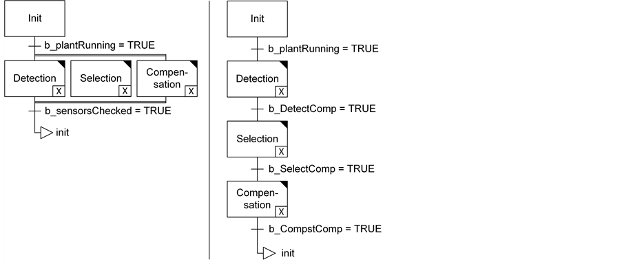
Figure 9. Different implementations for fault detection, selection and compensation.
With a sequential implementation of fault detection, selection and compensation (cp. Figure 9, right side), initially the time needed for fault detection (plcDFAI) has to be calculated according to (1.1). On the assumption that fault detection lasts one cycle (pcycles = 1) and the cycle time is adjusted to 30ms (tcycles = 30 ms), the plcDFAI also results in 30 ms.
The same is valid for fault selection, which is done in the next PLC-cylce. This again lasts one cycle time (icycles = 1) and the plcIFAI also results in 30 ms. After fault selection the fault compensation strategy is initiated. The initiation itself also lasts a cycle time (ncycles = 1)

The index for total real-time capability in the event of a fault (plcFCLAI) is then calculated with the single factors for real-time capability

By applying the metric for real-time capability to two different software implementations it was shown that the first variation (plcFCLAI = 30 ms) holds better real-time characteristics than the second implementation (plcFCLAI = 90 ms).
5.1.2. Metrics for Fault Coverage
In this section the metrics for fault coverage defined in Section 4.2 are applied to the introduced fault tree (cp. Figure 8) of the conveyor unit. At first the index BECAI (Basic Event Covered Adaptivity Index) is calculated according to (6). For this only the existing basic events of the fault tree are regarded. It is checked which basic events are measurable by the current PPU-configuration (factor c). This factor is divided by the total amount of existing basic events b. Thus, the BECAI results in:

With the current configuration of the system, 50% of the basic events are measurable.
The BENCAI (Basic Events Not Covered Adaptivity Index) amounts to 0.5 (50%), since 7 out of 14 basic events are not recordable by measurement techniques.

Since faults can be detected by the logical connection of basic events, the faults, that are detectable by registration with measurement techniques, are calculated. For this the index FLCAIj (Fault Level Coverage Adaptivity Index) for the level next above the basic events (j = 2) is determined. It is, therefore, necessary, to calculate how many faults are detectable based on the measurement technology. Applied to the fault tree, FLCAI2 (Formula (7)) results in:

Although 50% of the basic events are measurable, within the current configuration only one fault modeled in the fault tree is detectable, since only for this one fault (time constraint incorrect) all connected basic events are recordable. In order to increase the fault coverage it is necessary to adapt software and automation hardware as well as the mechanics of the PPU.
5.1.3. Metrics for the Programming Effort Needed to Increase Fault Coverage
In order to estimate the minimum effort to increase fault coverage, or rather to detect a fault, which can be turned into a measurable fault with a minimum amount of effort, the metrics defined in Section 4.3 are applied to the conveyor unit.
Initially, the fault modeled in the fault tree, which already has a very high amount of measurable basic events, is determined. For this the index MEICAI2 is applied. For all modeled faults on level 2 (j = 2), the amount of non-measurable basic events is divided by the total amount of modeled basic events. Subsequently, the value with the minimum ratio is selected. According to Formula (8) this leads to the following calculation:
At first the ratios are calculated for each fault on level 2.

Formula (1.8) requires the minimum ratio, whereby those MEICAI2, which equal zero, are excluded from further calculations. A zero is equivalent to a 100% metrological coverage of the basic events (cp. fault (6, 2)). Thus, the minimum MEICAI is fault (5, 2) with MEICAI2 = 0.33; which in the fault tree (cp. Figure 8) corresponds to a work piece jam through the pusher.
The effort for an extension of the software is expressed by the FHAI (cp. Formula (9)). In the function block diagram of the PPU (cp. Figure 10) inputs, outputs and function blocks have been retained as well as added or adapted. None of the software elements have been removed. Therefore, in this example only FHAInew, FHAIadapted and FHAIold (Formulas (10), (11), and (13)) are applied in order to calculate the FHAI.
Adaptations to FB_monitoring
FB_Monitoring in Figure 10 illustrates that inputs, outputs and function blocks have not been changed. Thus, only FHAIold has to be calculated which results in:

With i = 3 referring to the three inputs and o = 1 in accordance with the single output. The internal structure of FB_Monitoring has not been changed (fb = 1).
Adaptations to FB_monitoring_adaptive
The whole function block FB_Monitoring_adaptive has been newly added in order to process the new measured values and transfer the according fault status to FB_Fault_Hanlding. Thus, for this function block FHAInew

Figure 10. Software adaptation from the basic PPU configuration for detecting the fault work piece jam using self-configuration.
needs to be calculated. This results from the four newly added inputs (i = 4), two newly added outputs (o = 2) and the new function block FB_Monitoring_adaptive itself (fb = 1).

Adaptations to FB_fault_handling
FB_Fault_Handling includes new, adapted and also retained software elements. FAHIold results from the retained input (i = 1) and the retained output (o = 1). Thus it is calculated to

The newly added software elements (FHAInew) are, for once, the new inputs of the function block (i = 2) and also the newly added output (i = 1). The FHAInew results in

Since the internal structure of FB_Fault_Handling has been adapted, FHAIadapted results in

Overall effort of the software changes (FHAI)
Based on the previous calculations, it is possible to sum up the individual indexes FHAIold, FHAInew und FHAIadapted in order to calculate the overall effort of software adaptations (FHAI).


Thus the overall effort of software adaptations is calculated according to Formula (9) and results in

The FHAI is equal to 0.61 which means that overall 61% of the software elements need to be added or adapted. Thereby, internal structures such as the addition or adaptation of internal function blocks in Figure 10 are not included and would lead to an even higher overall effort.
5.1.4. Metrics for the Modeling Effort Needed to Increase Fault Coverage
In Figure 11, an excerpt of the PLC software based on plcUML [41] is given. In the manual mode (left hand side), the software is not able to identify a WP jam precisely and therefore triggers an alarm (201) if a product

Figure 11. Excerpt of plcUML state chart for manual and self-healing mode [16] .
does not reach the slide within the expected time (Timer t > 3 seconds). Obviously, this is a drastically simplified failure model. In contrast, the additionally installed sensors in the self-configuration case provide the necessary information to detect a WP jam more precisely. This failure can be exactly determined when (i) the transducer contained within the respective pusher indicates that it is not extended completely (sens_transducer), (ii) the pressure of the pneumatic system is not as expected (sens_pressure) and (iii) no WP entered the slide (sens_slide). According to [42] , automatic and manual mode is recommended in P&M. The self-configuration software functionality is realized as an additional functionality of the automatic operation mode. After detecting the fault and the corresponding failure, a sequence of operations for fault recovery, i.e. to remove the WP jam and the correct sorting of the WP, is executed (cp. Figure 11).
To detect the complexity of both plcUML state charts FHAImodel is applied. To calculate V(G)old all states are taken into account used in scenario 12 (cp. Figure 11, white, white-gray colored and initial and end state). Furthermore, all edges are counted that are related to a state from scenario 12. Resulting, 6 states and 6 transitions are realized for scenario 12. Hence, V(G)old is 2 regarding Formula (14).

An evolutionary plcUML implementation is also shown in Figure 11 (gray, white-gray colored and initial and end state). The new implementation is realizing the more precise fault detection, as mentioned above. There are 16 transitions and 19 states, resulting in a cyclometic complexity of 5

Using both results, FHAImodel can be calculated (Formula (15)) to get the relative complexity gradient as follows:

FHAImodel reveals to be about 0.857 indicating increasing complexity of the new plcUML implementation concerning the previous software evolution.
5.2. Restart of PPU after Emergency Shut-Down
In another part of the PPU shown in Figure 16, workpieces get stamped using two pneumatic cylinders. One of the pneumatic cylinders pulls the workpieces in to reach stamp position, one cylinder with adjustable pressure stamps the workpieces. In this case, the PPU is programmed using the adapted UML state charts for PLCs integrated within the CODESYS environment, which is introduced and explained in [41] (cp. Figure 12).
In a scenario during testing of the operation of the PPU the emergency stop is activated during stamping. When restarting after the emergency stop the PPU initializes its modules anew and starts operation beginning from a stack, where the workpieces are stored. When trying to stamp a workpiece the stamp has the old workpiece still in place, which collides with the new workpiece when the PPU tries to set the workpiece down. In order to eliminate this behavior a Failure Mode and Effects Analysis (FMEA) is conducted. An excerpt of the FMEA is shown in Figure 13. It is found that after initialization no analysis of the current state of the PPU and especially no analysis of workpieces that may still be within the PPU is done. Consequently, as a prevention, new conditions and more specifically transitions and one new state to firstly analyze the state of the PPU after start and restart and its workpieces is introduced.
In order to measure the effort required to implement identification of work piece positions after an emergency stop of the PPU, the complexity measure cyclomatic complexity measure V(G) by McCabe [40] (introduced in Section 4.4) is used. In order to implement the storing of work piece positions, only the state chart controlling the crane needs to be adapted. Depending on the position of a work piece after emergency stop, the crane needs to turn to the according station to resume the interrupted transport. The original state chart controlling the crane consists of 17 edges (e = 17), 15 states (n = 15) and only one state chart is needed to control the crane (p = 1). Thus, the V(G)old results in (cp. Formula (14)


Figure 12. PPU implementation of restart after emergency shut down as UML state chart implemented in CoDeSys V3 (dashed lines indicate added edges and elements).

Figure 13. Failure mode and effects analysis for collision of workpieces within stamp.
To enable the storing of work piece positions, an additional state as well as three additional transitions are necessary resulting in a state chart with a total of 20 transitions (e = 20) and 16 states (n = 16), while the number of analyzed state charts remains unchanged (p = 1). Therefore, the cyclomatic complexity measure V(G)new of the expanded crane state chart, according to Formula (14), calculates to

Overall, the cyclomatic complexity measure of the state chart increases by two when implementing the memorizing of work piece positions, which means (regarding Formula (15)) that the relative complexity measure (FHAImodel) increases by 0.4.

5.3. Self-Configuration with Model Based Redundancy for Liquid Level in Tank
For another example a tank, equipped with two sensors detecting the tank’s filling level (maximum and minimum), is considered. The tank is used to store liquids in a production process (cp. Figure 14). Once the minimum filling level of the tank is reached (detected by the lower tank sensor, sensor 101.2 in Figure 14), a valve (V101) is opened and the filling process starts. The filling process will run until the upper tank sensor (sensor 101.1) signals that the maximum filling level of the tank is reached. However, there is no redundancy in the process and, thus, a malfunction of the upper sensor leads to an overflow of the tank. As a precaution and in order to detect a failure of the upper sensor, the original tank function is enlarged by a self-configuration method according to Gronau’s classification of adaptivity [29] . For self-configuration the filling level of the tank is calculated based on the amount of fluid that is filled into the tank, the amount of fluid that flows out of the tank, the tank’s dimensions as well as the filling and emptying times. In the following, the introduced metrics to estimate the programming effort (cp. Section 4.3) are used to measure the effort of implementing this function on code level.
A transformation of the approach presented by Schütz et al. [17] into a fault coverage analysis tree (FCA) is presented in Figure 15. On the bottom of the FCA the basic events connected to a fault are shown, i.e. if inflow

Figure 14. Tank with upper and lower filling level sensors, valve and pump.

Figure 15. Part of a FCA regarding tank’s level control error.
or outflow or the level sensor is faulty, a filling level error and an inflow error and an outflow error would occur. As discussed above the real level sensor can be approximated by a virtual sensor (e.g. Figure 15, virtual filling level sensor) that is calculated during runtime and is added as basic event.
If the filling level sensor is effected by a fault as mentioned above, the faulty situation may be detected, but the reason for it remains unclear compared to the FCA in Figure 4 case study 5.1, e.g. the broken cable (electric fault), work piece jam (mechanical fault) or wrong software implementation (faulty software design). At first the redundancy model has to be developed in the design phase by taking functional dependencies into account formulated as physical equation. The redundancy model has to be implemented on the PLC to allow decisions during runtime. But nevertheless the approach allows only the self-configuration of one fault out of three real sensors and one calculated virtual one. BECAI may be calculated to 100% for filling level error neglecting physical reasons for such a fault, e.g. faulty cable, voltage, input channel etc. For level control error (j = 3), one out of three will be detected, resulting in:

5.3.1. Metrics for Real-Time Capabilities
In order to detect a malfunction of the upper sensor, no additional PLC cycle is necessary, since the filling level of the tank is calculated simultaneously to the normal program execution. Therefore, only cycle time is needed to detect a sensor failure (plcDFAI) and no additional time is needed to select (plcIFAI) and compensate (plcSTSAI) the calculated value compared to reacting to the actual sensor value, since the actual sensor value and the calculated value are checked at the same time (as two options in the same line of code). Thus, the metrics for real-time capabilities result in


Overall, the index for total real-time capability in the event of a malfunction of the upper tank sensor calculates to

5.3.2. Metrics for the Programming Effort Needed to Increase Fault Coverage
The original declaration part of the tank function (without self-configuration) consists of 14 lines of code (LOC) and the original implementation part consists of 22 LOC (not including comments). The whole declaration part and 21 LOC of the implementation part are retained in the new function (with self-configuration) and, thus, the FAHIold(calculates the unchanged software elements) adds up to

In order to implement self-healing, neither in the declaration part nor in the implementation part of the function LOC are removed (FHAIremoved = 0). Furthermore, in the declaration part of the self-healing function 8 LOC were added and in the implementation part 7 LOC were added. Therefore, the FHAInew is calculated as follows

Also, in the implementation part one LOC was modified to implement self-healing in the function (FHAIadapted = 1). Overall, the FHAI results to

This means in order to enlarge the function of the tank and thus detect and cover a failure of the upper tank filling sensor, 31 percent of the software code had to be modified or added.
5.4. Evaluation of Enhanced Recovery States Based on OMAC State Machine with xPPU
In order to evaluate the proposed metrics, another program (programmed by another engineer with a bachelor degree in computer science as well) with and without recovery function for the laboratory demonstrator xPPU is analyzed. The xPPU (cp. Figure 16) is an extension of the laboratory demonstrator introduced in Section 5.1. Work pieces are stored at the stack and, depending on their material, are either transported with the crane module to the stamping module before being sorted in the sorting unit (described in Section 5.1) or are directly transported to the sorting unit. Additionally to the features of the original PPU, the conveyor belt depicted in Figure 7 has been enlarged by a conveyor system, which enables re-feeding of work pieces from the original conveyor belt back into the manufacturing process and is also able to change the order of the work pieces.
The analyzed program is divided into unit modules, equipment modules and control modules according to the ISA88 physical hierarchy for code modules, which can be seen in Figure 17. The unit module is controlled by an OMAC state machine [15] (cp. Section 2 for description) thereby the active OMAC state calls the suitable function of the unit module. Subsequently, the suitable functions of the equipment modules are called by the unit module and the control modules by the associated equipment module. The return value of a function call is given as an enumeration (OPERATING, FINISHED, ERROR) which is an important part of the failure detection and recovery system. Additionally to the OMAC states and contrary to the traditional development process of field control software, the approach suggests the use of system states whereby machine capabilities are implemented as basic operations with pre- and post-conditions.
Therefore, additional auxiliary functions are needed for modeling the operations, pre- and post-conditions. To apply failure detection, the execution time of every basic operation is measured and used for the definition of a failure, which is defined as the exceedance of the average execution time of a basic operation by a chosen offset of 300ms. Thus the program of the PPU was enlarged by a recovery function, which enables the detection of a fault and transfers the plant into a recovery state.
Comparing the program described above to case study E, it is obvious that not only the architecture levels correspond to each other. Case study E likewise has got a system state given by its facility wide module control, yet with a more loose coupling to the architecture level below the module control, i.e. the modules in case study E. This allows a differentiated reaction to an error regarding the states of the modules. Nevertheless, like in the example shown in Figure 17, an occurring error in case study E also has an immediate influence on the state of its facility wide module control and thereby on the system state as the module control commands the states of all inferior modules.
In the following, the introduced metrics (cp. Section 4) are used to measure the adaptivity of the demonstrator program.

Figure 16. Picture of the extended Pick and Place Unit (xPPU).

Figure 17. Fault detection and transmission cascading through the architecture levels OMAC state machine, unit, equipment module (EM) and control module (CM).
5.4.1. Metrics for Real-Time Capabilities
In this section the real-time capability of this approach is analyzed. After initialization, the demonstrator program is executed in the state Execute. In order to monitor the fault-free execution of the program, the average time needed for the individual operations is measured during program execution. The considered failure is a false timing of the pusher-extraction, which is used for sorting the work pieces into slides. The failure may occur due to differences in conveyor speed and, therefore, a false timing between conveyor speed and pusher-extraction. Another reason for this failure can be the different friction behavior of the different types of work pieces. The failure is detected as follows: In case of fault-free execution the work piece to be sorted is detected by the according slide sensor (cp. Figure 7 sens_slide) after extracting the pusher. If however, the described timing fault occurs, the work piece is not correctly pushed into the slide and, therefore, the sensor sens_slide does not report the detection of a work piece. After the average time for the operation sort work piece is expired, an additional delay timer of 300 ms is started. This offset of 300 ms is chosen for the entire demonstrator to ensure that any action carried out by the demonstrator is definitely finished within the delay time. Once the failure is detected in the control module level, the return value ERROR is passed through the equipment and unit module level to the OMAC state machine and leads to a state transition to the OMAC state Holding (cp. Figure 17). The offset between the time, when a failure is detected, and the average execution time leads to a value of

In this state the program execution is stopped and the plant is transferred into a safe state. Once a safe state is obtained, the state is changed to Held and, for security reasons, no further actions are performed until the machine operator starts the recovery. Changing the state of the plant from Execute to Holding requires one cycle. Stopping the plant in a safe state and changing to the state Held, which completes the fault selection, takes at most two cycles. With a cycle time of 4ms (tcycles = 4 ms), the plcIFAI results in

Subsequently, the fault compensation strategy is started after completion of the fault selection. After an unknown time period toperator, which passes between fault selection and the operator’s user input to start recovery, the plant is transferred to the state Un-Holding in which automatic recovery is started. Once the operator’s input is detected, the initiation of the fault compensation is started either in the same cycle as the input or in the following cycle leading to a maximum time of two cycle times. In consideration of the unknown time period toperator, the plcSTSAI calculates to

The index for total real-time capability in the event of a fault (plcFCLAI) adds up to

By means of the metrics for real-time capability, different software implementations can be compared and the one with best real-time capability (lowest plcFCLAI-value) can be selected.
Since the analyzed program holds a recovery function for one fault only, the metrics for fault coverage are omitted in this example.
5.4.2. Metrics for the Effort to Increase Fault Coverage
The program is written in the programming language Structured Text. In order to measure the changes due to the addition of a recovery function, the metric Lines of Code (LOC) is applied. The total number of LOC of the overall program is 2511 without recovery function and in order to implement recovery, an additional 531 LOC are added. Thereby, the main function and the auxiliary functions are unchanged whereas every one of the modules has to be adapted.
The effort to implement recovery can be measured with the FHAI (cp. Formula (9)). In order to implement recovery for the fault “timing pusher”, no inputs or outputs were added, no lines of the original code were adapted and no parts of the code were removed. Therefore, FHAInew and FHAIold (Formulas (11) and (13)) are applied in order to calculate the FHAI.
Since the auxiliary functions and the main function have not been changed at all, only the metric FHAIinitial has to be calculated for those functions. The LOC of the main function and the nine auxiliary functions result in


Within the seven modules the LOCs of the original program were complemented by new LOCs, however, the original lines were not adapted. Thus, FHAInew and FHAIinitial need to be calculated for the module functions.


Overall, FHAInew and FHAIinitial add up to


Finally, the FHAI results in

This means that 17% of the software needed to be added in order to implement recovery from fault “timing pusher”.
Compared to the first programs (PRG A.1 and PRG A.2) analyzed in Section 5.1 (cp. Figure 9), the real-time capabilities of the program introduced in this section (PRG B) are significantly lower. Programs PRG A.1 and PRG A.2 have a plcFCLAI value of 30 ms and 90 ms, whereas PRG B has a value of (320 ms + toperator). However, this is mainly due to safety requirements prohibiting an automatic start of the recovery (toperator) and the chosen offset of 300 ms, which will be reduced in a future implementation. Since only one specific fault was considered in the OMAC program, no statement can be made about the metrics for fault coverage.
5.5. Results of the Evaluation
In this section the questions, whether the developed metrics are adequate to measure adaptivity in case of a fault and restart of an aPS after a shut down. The evaluation of the four scenarios showed that the wide range of all four scenarios could be measured reaching from self-configuration based on hardware adaptation, i.e. added sensors (add-on and modification according to Gronau’s classification), self-configuration on basis of virtual sensors to restartability after stop or emergency shut-down. The programming effort (fault handling adaptivity index) depends of course strongly on the numbers of faults being covered (cp. Table 2). Scenario 5.1 is the most sophisticated identifying the fault with redundant sensors, isolating it and automatically recovering by reversing
Table 2. Comparison of the metrics applied to the different application scenarios.
“-”: not applied.
the belt direction automatically to readjust the pusher and the work piece. Therefore, this scenario is the most challenging regarding the effort necessary to increase fault coverage, it includes restart (similar to 5.4). The other scenarios cover only limited aspects of the respective use case and therefore the effort is smaller, too. Scenario 5.3 only focuses on one fault and Scenario 5.2 and 5.4 only on the restart after an emergency shutdown or an inhibited work piece without identifying the reason of the fault.
Real time requirements are given by the technical process, which is controlled and have to be fulfilled. Same applies for metrics for real time capabilities to detect, isolate and compensate faults.
6. Conclusion/Summary/Outlook
Modularity has been identified as prerequisite for adaptive systems. This remains valid for Industry 4.0 or CPPS. The paper focuses on restart and self-configuration after a fault to increase OEE, i.e. to allow operation despite faulty devices and to detect and, isolate existing faults and adapt the machine or plant with self-configuration. Furthermore, the operator activities and interaction should be eased (cp 5.2 and 5.4). As a basis, eight use cases regarding fault handling from world market leading machine and plant manufacturing companies were introduced. Hierarchical fault handling is a frequent practice in special purpose machinery manufacturing as well as in plant manufacturing. The isolation of single faults and an automatic reaction to these faults needs to be implemented in order to be able to react to faults adaptively to reduce machine or plant shutdowns and additional manual interventions by operators in the future. In the domain of packaging plants for food & beverage, the OMAC state machine is already widely used which eases fault handling and restart (cp. 5.4 and case study E). Nevertheless, restart and self-configuration are limited due to the production process itself as well as redundant sensors or the availability of virtual sensors.
Selected metrics for adaptive automated Production Systems, selected metrics for real-time preservation in the event of a fault, fault coverage of a given automation system and the effort to extend the system, to increase fault coverage have been presented and evaluated with four scenarios ranging from no adaptation, adaptation add-ons, adaptation via modification to self-configuration. Future work will address on the one hand a more general challenge of software architecture of the effort to develop software for safety devices, e.g. protective covering as well as safety doors and on the other hand the development of more powerful metrics for adaptivity and Industry 4.0, which hopefully will allow to benchmark compliance of machine and plants to Industry 4.0.
Acknowledgements
We thank Professor Dr. H.C. Peter Göhner for his tireless commitment not just within FA 5.15 regarding the use of agents in automation and the successful realization of the demonstrator “MyJoghurt”. We thank the FA 5.15 Agents in Automation Technology for the discussion on the topic of metrics in Industry 4.0 and CPPS as well as the companies for providing an insight into their challenges and software structures concerning architectures and fault handling as well as restart and recovery after faults. We also thank the DFG Priority Program 1593 “Design For Future―Managed Software Evolution” for fruitful discussion and for partially funding this research within the project MoDEMAS (grand number VO 937/20-1).
Cite this paper
BirgitVogel-Heuser,SusanneRösch,JulianeFischer,ThomasSimon,SebastianUlewicz,JensFolmer, (2016) Fault Handling in PLC-Based Industry 4.0 Automated Production Systems as a Basis for Restart and Self-Configuration and Its Evaluation. Journal of Software Engineering and Applications,09,1-43. doi: 10.4236/jsea.2016.91001
References
- 1. Vogel-Heuser, B., Diedrich, C., Pantforder, D. and Gohner, P. (2014) Coupling Heterogeneous Production Systems by a Multi-Agent Based Cyber-Physical Production System. Proceedings of the 12th IEEE International Conference on Industrial Informatics (INDIN), Porto Alegre, 27-30 July 2014, 713-719.
- 2. VDI/VDE-Gesellschaft fur Messund Automatisierungstechnik (2015) Status Report Reference Architecture Model Industrie 4.0 (RAMI4.0). VDI e.V., Dusseldorf.
- 3. Vogel-Heuser, B., Fay, A., Schafer, I. and Tichy, M. (2015) Evolution of Software in Automated Production Systems—Challenges and Research Directions. Journal of Systems and Software (JSS), 110, 54-84.
http://dx.doi.org/10.1016/j.jss.2015.08.026 - 4. Jazdi, N., Maga, C. and Gohner, P. (2011) Reusable Models in Industrial Automation: Experiences in Defining Appropriate Levels of Granularity. Proceedings of the 18th IFAC World Congress, Milano, 28 August-2 September 2011, 9145-9150.
- 5. Feldmann, S., Fuchs, J. and Vogel-Heuser, B. (2012) Modularity, Variant and Version Management in Plant Automation—Future Challenges and State of the Art. Proceedings of the 12th International Design Conference (DESIGN 2012), Dubrovnik, 25 May 2012, 1689-1698.
- 6. Feldmann, S., Legat, C. and Vogel-Heuser, B. (2015) Engineering Support in the Machine and Plant Manufacturing Domain through Interdisciplinary Product Lines: An Applicability Analysis. Proceedings of the 15th IFAC Symposium on Information Control in Manufacturing (INCOM), Ottawa, 11-13 May 2015, 211-218.
- 7. Katzke, U., Vogel-Heuser, B. and Fischer, K. (2004) Analysis and State of the Art of Modules in Industrial Automation. ATP International-Automation Technology in Practice International, 46, 23-31.
- 8. Vogel-Heuser, B., Fischer, J., Rosch, S., Feldmann, S. and Ulewicz, S. (2015) Challenges for Maintenance of PLC-Software and Its Related Hardware for Automated Production Systems—Selected Industrial Case Studies. Proceedings of the 31st IEEE International Conference on Software Maintenance and Evolution (ICSME), Bremen, 29 September-1 October 2015, 362-371.
- 9. Vyatkin, V. (2011) IEC 61499 as Enabler of Distributed and Intelligent Automation: State-of-the-Art Review. IEEE Transactions on Industrial Informatics, 7, 768-781.
- 10. International Electronical Commission (2005) IEC International Standard IEC 61499-1: Function Blocks, Part 1: Architectures. IEC, Geneva.
- 11. Bonfè, M., Fantuzzi, C. and Secchi, C. (2013) Design Patterns for Model-Based Automation Software Design and Implementation. Control Engineering Practice, 21, 1608-1619.
http://dx.doi.org/10.1016/j.conengprac.2012.03.017 - 12. Guttel, K., Weber, P. and Fay, A. (2008). Automatic Generation of PLC Code beyond the Nominal Sequence. IEEE International Conference on Emerging Technologies and Factory Automation (ETFA), Hamburg, 15-18 September 2008, 1277-1284.
- 13. Barbieri, G., Battilani, N., and Fantuzzi, C. (2015). A PackML-Based Design Pattern for Modular PLC Code. IFAC-Papers on Line, 48, 178-183.
http://dx.doi.org/10.1016/j.ifacol.2015.08.128 - 14. Weihenstephan Standards. http://www.weihenstephaner-standards.de
- 15. OMAC. http://www.omac.org/content/packml
- 16. Vogel-Heuser, B., Legat, C., Folmer, J. and Rosch, S. (2014) Challenges of Parallel Evolution in Production Automation Focusing on Requirements Specification and Fault Handling. Automatisierungstechnik (at), 11, 755-826.
http://dx.doi.org/10.1515/auto-2014-1111 - 17. Schutz, D., Wannagat, A., Legat, C. and Vogel-Heuser, B. (2013) Development of PLC-Based Software for Increasing the Dependability of Production Automation Systems. IEEE Transactions on Industrial Informatics, 9, 2397-2406.
- 18. Bergagard, P., Falkman, P. and Fabian, M. (2015) Modeling and Automatic Calculation of Restart States For an Industrial Windscreen Mounting Station. Proceedings of the IFAC Symposium on Information Control Problems in Manufacturing (INCOM), Ottawa, 11-13 May 2015, 1030-1036.
- 19. Vogel-Heuser, B., Schutz, D., Frank, T. and Legat, C. (2014) Model-Driven Engineering of Manufacturing Automation Software Projects—A SysML-Based Approach. Mechatronics, 24, 883-897.
http://dx.doi.org/10.1016/j.mechatronics.2014.05.003 - 20. Priego, R., Schutz, D., Vogel-Heuser, B. and Marcos, M. (2015) Reconfiguration Architecture for Updates of Automation Systems during Operation. Proceedings of the 20th IEEE International Conference on Emerging Technologies and Factory Automation (ETFA), Luxembourg, 8-11 September 2015, 1-8.
- 21. Andersson, K., Lennartson, B., Falkman, P. and Fabian, M. (2011) Generation of Restart States for Manufacturing Cell Controllers. Control Engineering Practice, 19, 1014-1022.
http://dx.doi.org/10.1016/j.conengprac.2011.05.013 - 22. Andersson, K., Lennartson, B. and Fabian, M. (2010) Restarting Manufacturing Systems; Restart States and Restartability. IEEE Transactions on Automation Science and Engineering, 7, 486-499.
http://dx.doi.org/10.1109/TASE.2009.2034136 - 23. Bergagard, P. (2015) On Restart of Automated Manufacturing Systems, Ph.D. Dissertation, Department of Signals and Systems, Chalmers University of Technology, Goteborg.
- 24. Andersson, K., Richardsson, J., Lennartson, B. and Fabian, M. (2009) Coordination of Operations by Relation Extraction for Manufacturing Cell Controllers. IEEE Transactions on Control Systems Technology, 18, 414-429.
- 25. Bergagard, P. and Fabian, M. (2013) Calculating Restart States for Systems Modeled by Operations Using Supervisory Control Theory. Machines, 1, 116-141.
http://dx.doi.org/10.3390/machines1030116 - 26. Lennartson, B., et al. (2010) Sequence Planning for Integrated Product, Process and Automation Design. IEEE Transactions on Automation Science and Engineering, 7, 791-802.
http://dx.doi.org/10.1109/TASE.2010.2051664 - 27. Bengtsson, K., et al. (2012) Sequence Planning Using Multiple and Coordinated Sequences of Operations. IEEE Transactions on Automation Science and Engineering, 9, 308-319.
http://dx.doi.org/10.1109/TASE.2011.2178068 - 28. Ladiges, J., Fay, A., Haubeck, C. and Lamersdorf, W. (2013) Operationalized Definitions of Non-Functional Requirements on Automated Production Facilities to Measure Evolution Effects with an Automation System. IEEE International Conference on Emerging Technologies and Factory Automation (ETFA), Cagliari, 10-13 September 2013, 1-6.
- 29. Gronau, N., Lammer, A. and Andresen, K. (2007) Entwicklung wandlungsfahiger Auftragsabwicklungs systeme. GITO-Verlag, Berlin.
- 30. Wiendahl, H.-P., et al. (2007) Changeable Manufacturing—Classification, Design and Operation. CIRP Annals Manufacturing Technology, 56, 783-809.
http://dx.doi.org/10.1016/j.cirp.2007.10.003 - 31. Raibulet, C. and Masciadri, L. (2009) Towards Evaluation Mechanisms for Runtime Adaptivity: From Case Studies to Metrics. Computation World: Future Computing, Service Computation Cognitive, Adaptive, Content, Patterns, Athens, 15-20 November 2009, 146-152.
http://dx.doi.org/10.1109/computationworld.2009.89 - 32. Fischer, J., Friedrich, D. and Vogel-Heuser, B. (2015) Configuration of PLC Software for Automated Warehouses Based on Reusable Components—An Industrial Case Study. Proceedings of the 20th IEEE International Conference on Emerging Technologies and Factory Automation (ETFA), Luxembourg, 8-11 September 2015, 1-7.
- 33. German Institute for Standardization—DIN Deutsches Institut fur Normung e. V. (1985) DIN 25419: Event Tree Analysis; Method, Graphical Symbols and Evaluation. DIN, Berlin.
- 34. Friedrich, A. and Gohner, P. (2015) Fault Diagnosis of Automated Systems Using Mobile Devices. Proceedings of the 20th IEEE International Conference on Emerging Technologies and Factory Automation (ETFA), Luxembourg, 8-11 September 2015, 1-8.
- 35. Fuchs, J., Feldmann, S., Legat, C. and Vogel-Heuser, B. (2014) Identification of Design Patterns for IEC 61131-3 in Machine and Plant Manufacturing. Proceedings of the 19th IFAC World Congress (IFAC 2014), Cape Town, 24-29 August 2014, 6092-6097.
- 36. Vogel-Heuser, B. (2014) Usability Experiments to Evaluate UML/SysML-Based Model Driven Software Engineering Notations for Logic Control in Manufacturing Automation. Journal of Software Engineering and Applications, 7, 943-973.
http://dx.doi.org/10.4236/jsea.2014.711084 - 37. Frey, G., Litz, L. and Klockner, F. (2000) Complexity Metrics for Petri Net Based Logic Control Algorithms. IEEE International Conference on Systems, Man, and Cybernetics, Nashville, TN, 8-11 October 2000, 1204-1209.
http://dx.doi.org/10.1109/icsmc.2000.886016 - 38. Chidamber, S.R. and Kemerer, C.F. (1994) A Metrics Suite for Object Oriented Design. IEEE Transactions on Software Engineering, 20, 476-493.
http://dx.doi.org/10.1109/32.295895 - 39. Michura, J. and Capretz, M.A.M. (2005) Metrics Suite for Class Complexity. IEEE International Conference on Information Technology: Coding and Computing (ITCC), Las Vegas, NV, 4-6 April 2005, 404-409.
http://dx.doi.org/10.1109/itcc.2005.193 - 40. McCabe, T.J. (1976) A Complexity Measure. IEEE Transactions on Software Engineering, SE-2, 308-320.
http://dx.doi.org/10.1109/TSE.1976.233837 - 41. Witsch, D. and Vogel-Heuser, B. (2011) PLC-Statecharts: An Approach to Integrate UML-Statecharts in Open-Loop Control Engineering—Aspects on Behavioral Semantics and Model-Checking. Proceedings of the 18th IFAC World Congress, Milano, 28 August-2 September 2011, 7866-7872.
- 42. German Institute for Standardization—DIN Deutsches Institut fur Normung e. V. (2009) DIN EN 13128: Safety of Machine Tools—Milling Machines (Including Boring Machines). DIN, Berlin.
Appendix A. Software Code Example Self-Configuration Tank (Section 5.3)
LOC marked with comment //SHM were added or adapted in order to implement self-configuration to the function. Adapted LOC are furthermore marked with the comment (*SHM*) within the line, indicating the adapted parts in the line.
Declaration
Implementation
Appendix B. Extract from Software Code Example Recovery (Section 5.4)
The source file main is the entry point of the program. It handles the OMAC State Machine and the switch between unit modes.
Main
The method execute from the class pickAndPlaceUnit is called in the OMAC State Machine defined in main. The method is repsonsible for executing the graph and detection of failures on the unit level.
pickAndPlaceUnit.execute()
The equipment module sorting plant is called from the unit module pick and place unit as described with the physically hierarchy.
sortingPlant.execute()
The equipment module sorting plant calls the execute method of the control module conveyor.
conveyor1.execute()
After detecting a failure in the control module conveyor, the return values of the methods are tERROR, which leads to an OMAC state change to HOLDING. In HOLDING the machine is stopped and transferred in a safe state. Subsequently, the OMAC State Machine changes the state to HELD. After pressing the start button, the OMAC State UNHOLDING is active. In this state the failure recovery is performed.
pickAndPlaceUnit.unholding()
The Pick and Place Unit calls the method unholding of the equipment module sorting plant.
sortingPlant.unholding()
The equipment module sorting plant calls the method unholding of the control module conveyor. The failure recovery is performed. Subsequently, after the failure recovery, the OMAC State Machine switches to the OMAC State EXECUTE.
conveyor1.unholding()