Journal of Biomedical Science and Engineering
Vol.10 No.03(2017), Article ID:74662,30 pages
10.4236/jbise.2017.103008
Providing a Therapeutic Scheduling for HIV Infected Individuals with Genetic Algorithms Using a Cellular Automata Model of HIV Infection in the Peripheral Blood Stream
Gelayol Nazari Golpayegani1, Amir Homayoun Jafari2,3*, Nader Jafarnia Dabanloo1
1Department of Biomedical Engineering, Science and Research Branch, Islamic Azad University, Tehran, Iran
2Medical Physics and Biomedical Engineering Department, School of Medicine, Tehran University of Medical Science, Tehran, Iran
3Research Center for Biomedical Technologies and Robotics (RCBTR), Tehran University of Medical Sciences, Tehran, Iran

Copyright © 2017 by authors and Scientific Research Publishing Inc.
This work is licensed under the Creative Commons Attribution International License (CC BY 4.0).
http://creativecommons.org/licenses/by/4.0/


Received: May 6, 2016; Accepted: November 10, 2016; Published: March 13, 2017
ABSTRACT
The aim of this study is to develop two-dimensional cellular automata model of HIV infection that depicts the dynamics involved in the interactions between acquired immune system and HIV infection in the peripheral blood stream. The appropriate biological rules of cellular automata model have been extracted from expert knowledge and the model has been simulated with determined initial conditions. Obtained results have been validated through comparing with the accepted AIDS reference curve. The new rules and states were added to the proposed model to show the effects of applying combined antiretroviral therapy. Our results showed that by applying RTI and PI drugs with maximum drug effectiveness, comparing with cases in which no treatment was applied, the steady state concentrations of healthy (infected) CD4+T cells were increased (decreased) 53% (41%). Also, the use of cART with maximum drug effectiveness led to a 69% reduction in the steady state level of viral load. At this time, obtained results have been validated through comparing with available clinical data. Our results showed good agreement with both reference curve and the clinical data. In the second phase of this study, by applying genetic algorithms, a therapeutic schedule has been provided that its use, while maintaining the quality of the treatment, leads to a 47% reduction in both drug dosage and the side effects of antiretroviral drugs.
Keywords:
HIV Infection, Cellular Automata Model, Combined Antiretroviral Therapy, Genetic Algorithms

1. Introduction
Human Immunodeficiency Virus (HIV) is a subgroup of retrovirus that causes the Acquired Immune Deficiency Syndrome (AIDS), a condition in humans in which progressive failure of the immune system allows life-threatening opportunistic infections and cancers to thrive. HIV infects vital cells in the human immune system such as helper T cells (specifically CD4+T cells), macrophages and dendritic cells [1] . Figure 1 shows HIV life cycle. According to the World Health Organization, millions of people die each year from Acquired Immune Deficiency Syndrome (AIDS) [2] . That’s why most of research teams have focused their studies on AIDS and their knowledge about Human Immunodeficiency Virus (HIV) has been improved significantly. Although AIDS is not treatable definitely, it is controllable [3] . Antiretroviral drugs have been effectively applied to control the progression of disease in the HIV infected individuals because they increase the time interval between entry of HIV and onset of AIDS. Two of the most important categories of antiretroviral drugs for AIDS control are Reverse Transcriptase Inhibitors (RTI) and Protease Inhibitors (PI). The RTI antiretroviral drugs interfere with ability of HIV enzyme reverse transcriptase to convert HIV RNA into HIV DNA. Thus they can stop the HIV replication process. The PI drugs prevent the assembly of particles of new virus by interfering with HIV enzyme protease. Since by transforming the HIV as a result of mutation, some strains of HIV will be resistant to the type of drug used, therefore, the chance to control the HIV will be increased if the patient uses multiple types of drugs simultaneously. One of the conventional methods in HIV control is Combined Anti Retroviral Therapy (cART) in which the patient uses combination of RTI and PI antiretroviral drugs [4] .

Figure 1. HIV life cycle. This figure is available online in www.Southsudanmedicaljournal.com
By finding an appropriate model for a biological system, experts will be needless to do many relevant clinical trials. If we also consider the effects of drug therapy in such models, we will be able to introduce the best treatment by simulating the effects of different therapeutic methods. Although antiretroviral therapy has significant effects on prolonging survival of patients, the side effects of long-term applying of these drugs may put the patient at risk [5] . Therefore, in this study, after development of an appropriate model of HIV infection in the peripheral blood stream of patients who are submitted to antiretroviral therapy, a therapeutic schedule is provided that its use causes to a significant decrease in drug dosage. As a result, by applying obtained therapeutic schedule, while maintaining the quality of treatment, the side effects of antiretroviral drugs will be decreased significantly.
Most of researchers have used models with Ordinary Differential Equations (ODEs) or Partial Differential Equations (PDEs) to simulate the dynamics of HIV infection [6] [7] [8] . The biological systems such as human immune system are so complicated and their components interact with each other through specific rules that are almost impossible to depict such rules using ODEs approach. On the other hand, ODEs modeling approaches are unable to depict the specific properties of immune systems such as memory and emerging [9] . Also, especially when the drug is administered to control the disease, behavioral variations, and special states arise which ODEs modeling approaches are unable to depict all of these variations and they can’t consider appropriate parameters for showing all of these states. Because of the reasons mentioned, in this study, instead of using ODEs approaches we tried to use a qualitative modeling method based on rules to simulate the complicated and nonlinear dynamics of a human immune system and its response to the virus entered the human body.
The Cellular Automata (CA) modeling approach is a perfect choice for this type of modeling techniques. Cellular Automata (CA) is discrete dynamical systems for which its behavior is based entirely on local communications [10] . The main idea of CA is that each region of grid is considered as a cell, and specific status is assigned to that cell. In each iteration, the state of each cell will be updated, according to own state and the neighboring cells state. The neighboring cells of one cell include the cell itself and its nearest adjacent cells. These states are correlated to each other through certain rules. These rules are obtained from the biological and physical rules which are responsible for guiding the system behavior. Since in most biological systems a large degree of uncertainty is observed, therefore, for such systems, using the deterministic rules is not reasonable. Thus in modeling the biological systems with CA method, sometimes it will be necessary to consider probable rules [11] . CA modeling power is from its simplicity and at the same time its ability to model complex systems. Also, due to the direct use of real biological rules governing the issue, there will be the possibility of full compliance of model to the reality of issue [12] . Some researchers have developed different CA models to explain the dynamics of HIV infection and most of them have focused on lymphoid tissue. Dos Santos used two-di- mensional CA modeling approach to model the dynamics of HIV proliferation and infection in the lymphoid tissue [12] . They dispersed a fraction of infected CD4+T lymphocytes as the initial infection among of the healthy CD4+T lymphocytes and depicted the interactions between these healthy and infected lymphocytes through a set of simple rules. Then they validated their model through comparing the behavioral quality of their obtained results with a reference curve which shows the natural history of HIV infection dynamics currently accepted. This common pattern is depicted in Figure 2. The study was conducted by dos Santos was the basis of many articles published in the field of modeling the dynamics of HIV infection in lymphoid tissue using CA approach [13] [14] [15] [16] .
In the previous mentioned literature, the dynamics of HIV infection have been studied in the lymph node. However, whenever most physicians try to assess the progress of disease, they would prefer to use patient’s blood data because such data can be accessed more easily. Moreover, they can find all types of cells in the peripheral bloodstream. Because of these reasons, some of the authors selected peripheral bloodstream to model the dynamics of HIV infection using CA method [17] [18] . Jafelice et al. developed a CA model to simulate the evolution of HIV in the bloodstream of positive individuals [17] . They studied the effects of drug therapy in their model using a fuzzy rule based system with two inputs, the medication potency and patient’s treatment adhesion. They considered four types of cells namely uninfected cells, infected cells of lymphocytes T of CD4+, free virus particles and specific antibodies CTL. These cells were placed at random positions initially in a two dimensional cell grid and the states of each cell in the grid were updated according to the defined local dynamic rules of each cell. Obtained results were validated through the reference HIV history pattern. It should be noted that their work was invaluable but they just had considered cellular response of immune system and they ignored the role of humoral response in the adaptive system. Moreover, the effects of intracellular biochemical factors that influence the effectiveness, such as the susceptibility of inhibiting

Figure 2. The natural history of HIV infection dynamics currently accepted [18] .
drugs was not considered. Khabouze et al., developed the study done by Jafelice by taking into account the role of humoral response as one of the basic part of adaptive immune system by considering a new type of cell called antibody but the effects of drug treatment in their model was not studied [18] .
In this study we model the interactions between HIV enters the human’s body and the immune system response, in the peripheral bloodstream, using two-dimensional CA technique. We also consider the effects of antiretroviral therapy in our model rules. Actually our CA model is an extended version of model proposed by Khabouze [18] by taking into account the following important points: a) the effects of either mono or combined antiretroviral therapy. For this purpose we considered new cell states associated with reverse transcriptase inhibitors and protease inhibitors drug absorption by the healthy cells of CD4+T lymphocytes and we defined new rules to show how these inhibitor drugs can prevent the healthy cells from infection. We also investigated the effects of drug efficiency and initial time of onset of treatment in improving the quality of treatment. b) The phenomenon of drug resistance, c) The effect of latently infected cells in clinical latency phase of HIV infection and their important role in taking the patient to the onset of AIDS phase, d) The phenomenon of virus mutation, e) Infecting the healthy cells through contact with either free viruses or infected cells, while in the previous studies [17] [18] , authors considered that infection of healthy cells can only occur through free viruses. The simulation results obtained from our CA model reproduces three phase pattern of HIV infection and shows how the use of antiretroviral therapy is able to delay the arrival of the patient to the onset of AIDS phase. We validated our results through comparison with available clinical data.
In the next step, we used an intelligent optimization technique to provide an optimal therapeutic schedule that simultaneously keeps disease progression under control and allows the restoration of immune system. So far, in often models that have been used to depict the dynamic behavior of HIV, the time-continuous equations have been applied, and in this case, using optimal control methods (despite the high computational volume) were the best treatment strategy. However, since the CA model that used in this study is described by biological rules and there is no analytical equation, applying the classic optimal control methods is impossible. Therefore, in order to optimize treatment protocol and to provide optimal therapeutic schedule in terms of number and order of days of applying antiretroviral drugs and drug dosage, utilizing of algorithms which are search-based in discrete-time space, is recommended. Since the genetic algorithm is a good candidate of such algorithms, in this study we used genetic algorithms to provide the optimal therapeutic schedule.
After this introduction, this paper is organized as follow: in the next section, we introduce the proposed CA model by incorporating the antiretroviral therapy process into the rules of this model. Then we present the simulation results and we compare our obtained results with available clinical. After ensuring the validity of proposed model, in the next step, by utilizing the genetic algorithms, the optimal therapeutic schedule is obtained. In order to prove the effectiveness of the proposed treatment program, the results obtained from applying this optimum schedule is compared with the results obtained from two other therapeutic programs named “Full therapy” and “Random therapy”, respectively. In the last section we have concluded our work and suggestions for future works are expressed.
2. Material and Methods
2.1. Proposed Cellular Automata Model
The structure of proposed model in this study is two-dimensional CA model with Moor neighboring. For developing such a structure, we used two-dimen- sional cell grids with size of 250 × 250 to depict the bloodstream toroidal system.
Since CA models belong to subset of agent based modeling methods, defining the agents of proposed CA model is the first step of organizing this model. In this study, following agents have been defined:
1) Healthy cells (H): this is the state of a normal healthy cell which has not absorbed any type of antiretroviral drugs. The cell in this state is capable of becoming infected and this happens, it can infect other healthy cells in own neighboring.
2) Healthy cells resistant to infection (HR): this is the state of healthy cells in which due to the absorption of both RTI and PI antiretroviral drugs, they will not become infected even if they are exposed to infectious factors.
3) Active infected cells (A1): this state refers to the active infected cells which are able to infect the normal healthy cells in their own neighboring [12] .
4) Inactive infected cells (A2): this state corresponds to the infected cells that after Ƭ1 time delay, the immune system has developed own cellular response against it. With considering such time delay we can depict the mutation rate of HIV. In fact we consider that since each infected cell contains a new strain of HIV, thus the immune system needs time to identify each of them. On the other hand, as a result of cellular response of immune system, such infected cells alone are not able to infect the normal healthy cells in their own neighboring but local aggregation of them will cause the neighbor healthy cells to become infected. It means that if, at least, R numbers of A2 cells have been located in the neighboring of a normal healthy cell, the healthy cell will become an active infected cell [12] .
5) Latently infected cells (A0): this is the state of infected cells which have kept the latent infection in to themselves for a time and they are not capable of spreading the infection during this period of time. But they may be re-activated after a time delay Ƭ2 and if it happens, they will be able to infect their own adjacent healthy cells [14] .
6) Inactivated infected cells in effect of PI drug absorption (API): this state corresponds to the infected cells which have arisen due to infecting healthy cells that have absorbed PI antiretroviral drugs. The cells in this state are not able to spread the infection and they will not produce any new HIV strain.
7) HIV Infectious: this is the state of active and infectious HIV particles which are capable of infecting their own adjacent normal healthy cells [16] .
8) HIV non-Infectious: when a healthy cell that has absorbed PI antiretroviral drugs becomes infected, this type of infected cell produces free viruses that are often defective and are not capable of infecting other healthy cells. This state is corresponds to such detective and non-infectious viruses [16] .
9) HIV Inactive: this state corresponds to viruses that the immune system has developed own humoral response against them. Therefore, due to the performance of immune system, the ability of such viruses is decreased for infecting other healthy cells [16] .
10) Dead cells (D): this state corresponds to both of the healthy cells and free viruses that are dead due to natural death. This state also contains the infected cells that will die in next step due to the performance of immune system against them [12] .
11) CTLs: the state of immune system cells that is responsible for identifying killing the infected cells [17] .
12) Anti bodies (AB): the state of anti bodies that are responsible for killing the viruses [18] .
In second step, we considered following percentages as an initial number of each of cell types in our model: 25% ± 10% of the entire cell grid was initially considered as normal healthy CD4+T lymphocytes [17] [18] . To depict the initial infection, we considered 0.05% of the entire cell grid as infected cells [12] . 5% ± 1% of the entire cell grid was considered as free infectious viruses [17] [18] . CTLs and anti bodies, each of them initially constituted 3% ± 1% of the entire cell grid [18] . Mentioned cells, initially were randomly distributed in the cell grid space.
2.1.1. The Rules of Proposed CA Model
As previously mentioned, in this study we have developed a CA model for modeling the HIV infection in the peripheral bloodstream with taking into account the effects of applying antiretroviral therapy. For this purpose, the effectiveness of RTI and PI drugs was considered by PRTI and PPI, respectively, and the value of them was selected between 0 to 0.9 (the value of 0 indicates no use of drug of interest and the value 0.9 indicates maximum effectiveness of the drug). We defined following rules for our proposed CA model based on neighboring. It is worth noting that in the defined rules where ever the phrase “in the presence of infecting factors” is used, it means that, at least, one active infected cell (A1) or one infectious HIV or R numbers of inactivated infected cells (A2) exist in the neighborhood of target cell.
Rule 1) The rules for updating the state of a normal healthy cell (H):
a) We have defined a lifespan limit for normal healthy cells and a random initial age (between 0 and the lifespan limit) has been assigned to each of H cells. At the beginning of each of iterations, if an H cell reaches its lifespan then it will die, otherwise the following updating rules will be used [17] [18] .
b) The H cell will choose randomly an empty place in the neighborhood and moves there for the next iteration. If there is no empty place then it remains at own place [17] .
c) For the next iteration, each of H cells, becomes an HR cell with probability of PRTI×PPI in the presence or absence of infecting factors―it shows that when a normal healthy cell absorbs both of RTI and PI drugs simultaneously, it becomes a resistant healthy cell which none of the infecting factors are not able to infect that and it is protected from infection for longer period of time than the normal healthy cells which have absorbed only RTI drug;
Or remains an H cell with probability of PRTI × (1 − PPI) in the presence or absence of infecting factors and its age will be increased one unit?this shows that if a normal healthy cell only absorbs RTI drug, in the effect of this type of drug the virus prevents from entering to healthy cell. So the healthy cell will be protected from infection, but since it has not absorbed both RTI and PI drugs, this protection lasts only until the next iteration-;
Or with probability of (1 − PRTI) × PPI, two modes may occur: 1) in the absence of infecting factors, it remains an H cell and its age will be increased one unit, 2) in the presence of infecting factors, it becomes an AP cell with age zero?it shows that since the healthy cell has not absorbed RTI drug, it will not protected from entering virus and, therefore, it will be infected in presence of infecting factors. But since it has absorbed PI drug, even if it becomes infected by infecting factors, the risen infected cell (API) will not be able to infect other healthy cells-;
Or with probability of (1 − PRTI) × (1 − PPI) two modes may occur: 1) in the absence of infecting factors it remains at H state and its age will be increased one unit for the next iteration, 2) in the presence of infecting factors it becomes an active infected cell (A1) with age of zero with probability of Pinf, or it becomes a latently infected cell (A0) with age of zero with probability of (1 − Pinf) [14] [15] .
d) The normal healthy cells are proliferating with a constant rate during the simulation [17] [18] .
Rule 2) The rules for updating the state of a resistant healthy cell (HR):
Since a resistant healthy cell has absorbed both of RTI and PI drugs, therefore, even if the infecting factors exist in its neighborhood, it will not become infected. This type of healthy cell becomes a normal healthy cell for the next iteration [15] [16] .
Rule 3) The rules for updating the state of active infected cells (A1):
If an A1 cell is not identified by the immune system cells, it releases a new infectious HIV from within itself with probability of PHIV-PR [16] [18] [19] . According to empirical findings, each of active infected cells may be identified by effective immune cells about 3 to 5 weeks after infection and loses its ability to spread the infection and becomes an inactivated infected cell (A2) [12] [19] . In the previous studies, the time required to identify A1 cells by the immune system cells was considered 4 weeks (the average of 3 and 5 weeks) [12] . But in this study, instead of averaging, we considered that there is the probability of identifying an A1 cell by the immune system cells during the third until fifth weeks after infection of healthy cell. From the third week until fifth week, this probability is increasing. But due to the occurrence of mutation, an infected cell may contain a new strain of HIV into itself which has not previously been introduced to the immune system. For this reason, an infected cell may not be identified by the immune cells even five weeks after occurrence of infection. In this case, due to release of several HIVs from infected cell, its membrane will tear and thus the infected cell becomes dead cell for the next iteration [20] .
The state of A1 cell is updated according to the following rules:
a) Until three weeks after infection, an A1 cell produces HIVInfectious with probability of PHIV-PR or produces HIVInactive with probability of (1-PHIV-PR) for the next iteration. The new released HIV is placed at one of empty sites in A1’s neighborhood. Also the age of an A1 cell is incremented one unit for the next iteration [16] [18] .
b) Between three until five weeks after infection, following modes may occur:
1) If there is, at least, one CTL in the neighborhood, for the next iteration, an A1 cell becomes A2 with probability of Pidentification; or produces HIVInfectious with probability of (1 − Pidentificatin) × PHIV-PR; or produces HIVInactive with probability of (1 − Pidentificatin) × (1 − PHIV-PR). Also the age of an A1 cell is incremented one unit for the next iteration [12] [16] [17] [18] [19] .
2) If there is no CTL in the neighborhood, for the next iteration, an A1 cell produces HIVInfectious with probability of PHIV-PR; or produces HIVInactive with probability of (1-PHIV-PR). Also the age of an A1 cell is incremented one unit for the next iteration [16] [18] .
c) If due to mutations, an A1 cell is not detected by the CTLs up to five weeks after infection, due to releasing new viruses from within it, finally the cell membrane of this A1 cell will tear and it will die for the next iteration [20] .
d) Before an infected cell dies due to membrane rupture, if it is not detected at each of iterations by CTLs then for the next iteration it will select randomly an empty place in its neighborhood to move there and the age of this A1 cell is incremented one unit. But if there is no empty place in its neighborhood then it remains at an own place and its age is incremented one unit for the next iteration [17] [18] .
Rule 4) The rules for updating the state of an inactivated infected cell (A2):
An A2 cell becomes a dead cell for the next iteration [12] .
Rule 5) The rules for updating the state of a latently infected cell (A0):
a) Each of A0 cells after a time delay TRe-activation will be reactivated with probability of PRe-activation and becomes a new A1 cell with the age of zero for the next iteration; or remains an A0 with probability of (1 − PReactivation) and dies for the next iteration [14] .
b) Before reaching the time of TRe-activation, for the next iteration each of A0 cells will randomly select an empty place in its neighborhood to move there and if there is no empty place, it remains at own place. Also the age of A0 cell is incremented one unit for the next iteration.
Rule 6) The rules for updating the state of an API cell:
As we mentioned before, whenever a healthy that has absorbed PI drugs becomes infected by infecting factors in its neighborhood, it becomes an API cell with the age of zero for the next iteration. We also considered a lifespan limit for API cells similar to what we had previously defined for A1 cells (5 iterations). We defined following rules for updating the state of API cells:
a) If an API cell reaches its lifespan limit, it becomes a dead cell for the next iteration.
b) Before reaching the lifespan limit, following modes may occur for the next iteration:
1) It remains an API cell and produces HIVnoninfectious with probability of PPI × PHIV-PR; or it remains an API cell and produces HIVInactive with probability of PPI × (1 − PHIV-PR). The new released HIV is placed at one of the empty sites in API’s neighborhood. In this case, the API cell will randomly choose an empty place in the own neighborhood to move there and if there is no empty place, it remains at own place. Also the age of API cell is incremented one unit for the next iteration.
2) It becomes an A1 cell with the last age of API cell and produces HIVInfectious with probability of (1 − PPI) × PHIV-PR; or it becomes an A1 cell with the last age of API and produces HIVInactive with probability of (1 − PPI) × (1 − PHIV-PR). In this case, as we mentioned before, the arisen A1 cell continues its life with the last age of corresponding API cell and from now on, the rules that were defined for updating the state of A1 cell will be used for it.
The rules defined for updating the state of API cell is inspired from [4] [21] .
It is worth mentioning that the viruses which are produced by API cells or by A1 cells will be placed randomly in one of the neighboring places of infected cell producing their own. Depending on the type of the selected place, following modes may occur:
I. If this place is an empty place then the produced virus will be located there for the next iteration.
II. Since only the normal healthy lymphocytes are hosts for viruses, thus if this place be relevant to any state except H, the virus will not have no effect on the state of the place.
III. If this place is relevant to a normal healthy cell, since both of HIVnon-Infectious and HIVInactive are not capable enough to infect other cells, thus only HIVInfectious particles can infect the H cell.
Rule 7) The rules for updating the state of dead cells:
A dead cell can be replaced by a new healthy cell for the next iteration. The probability of this replacement is shown by Preplication. In fact, Preplication depicts the ability of the immune system for reconstructing the destroyed cells. Among new produced healthy cells, a very small fraction of them contain the infection. The new produced cell may be infected with probability of Pnew-infection [12] . Therefore, following rules have been defined for updating the sate of dead cells:
a) Each of dead cells becomes a new normal healthy cell (H) with probability of Preplication × (1 − Pnew-infection) or becomes a new infected cell (A1) with probability of Preplication × Pnew-infection or remains a dead cell with probability of (1 − Preplication) for the next iteration [12] .
Rule 8) The rules of HIV proliferation and updating its state:
As mentioned before, HIVInfectious is a virus particle that is able to infect own adjacent healthy cells. It means if there is, at least, one HIVInfectious in the neighborhood of a normal healthy cell, this virus transcribes own RNA in to the DNA of host cell through reverse transcriptase enzyme and infect the healthy cell in this way. On the other hand, the rules numbers 3a, 3b and 6b show how one A1 or API cell causes to the proliferation of this type of HIV. We also defined following rules for updating the state of HIVInfectious:
a) We defined a lifespan limit for HIVInfectious particles that is shown by the parameter “V_LSL”. If one HIVInfectious particle reaches the V_LSL, this virus particle will die due to the natural death for the next iteration [16] [17] [18] .
b) Before the HIVInfectious reaches V_LSL, following modes may occur:
1) At each iteration, if there is, at least, one anti body cell (AB) in the neighborhood of an HIVInfectious and detects this HIV particle with probability of Pidentification then the HIVInfectious will lose its ability for spreading the infection due to the performance of humoral response of immune system. Therefore, the HIVInfectious becomes HIVinactive for the next iteration [16] [18] [20] .
2) If the HIVInfectious is not identified by the AB cell in its adjacent with probability of (1 − Pidentification), or if there is not any AB cell in the neighborhood of this HIVInfectious, then for the next iteration the HIVInfectious will randomly select one of the empty places in own neighborhood to move there and if there is no empty place, it will remain at own place. Also, the age of this HIVInfectious is incremented one unit for the next iteration [18] [20] .
As mentioned before, whenever a normal healthy cell that has absorbed PI drugs, becomes infected by infecting factors, the arisen infected cell (API) produces the HIV particles which are often faulty and are not able to infect other healthy cells. We called this type of HIV particles HIVnon-infectious. The rule 7b shows how API cells produce this type of HIV. We also defined following rule for HIVnon-infectious:
c) Each of HIVnon-infectious becomes HIVinactive for the next iteration [16] .
Also we defined following rule for HIVinactive:
d) Each of HIVinactive becomes a dead cell for the next iteration [16] .
Rule 9) The rules for updating the state of CTLs:
The immune system develops own cellular response against infection through CTLs. This type of immune system cell is responsible for killing the infected cells. The rule number 3 shows how CTLs detect the infected cells and kill them. Following rules has been defined for updating the state of CTLs:
a) A lifespan limit for CTLs (CTL_LSL) has been defined. If a CTL reaches the lifespan limit then it becomes a dead cell for the next iteration. Otherwise, for the next iteration it will randomly select an empty place in the own neighborhood to move there and if there is no empty place then it remains at own place. Also, the age of CTL is incremented one unit for the next iteration [17] [18] .
b) At each of iterations, CTLs are being reproduced by a constant rate (CTL_PR).
Rule 10) The rules for updating the state of anti bodies:
The main role of antibodies (AB) is identifying virus particles and killing them. In rule 8b, we described how AB cells do this task. Following rules has been defined for updating the state of AB:
a) A lifespan limit for AB cells (AB_LSL) has been defined. If an AB reaches the lifespan limit then it becomes a dead cell for the next iteration. Otherwise, for the next iteration it will randomly select an empty place in the own neighborhood to move there and if there is no empty place then it remains at own place. Also, the age of AB is incremented one unit for the next iteration [18] .
b) At each of iterations, AB cells are being reproduced by a constant rate (AB_PR).
Figure 3 shows the block diagram of the interaction between the states of all agents.
2.1.2. The Parameters of Proposed Model
In order to simulate the proposed model, we used a set of parameters some of which have been extracted from reference articles and the rest of them are derived from expert knowledge and experimental findings. The expert knowledge includes medical reference books on AIDS [22] [23] , medical authoritative articles on AIDS [19] [20] [24] [25] [26] [27] and knowledge of infectious disease specialist. Table 1 shows the value of parameters used for simulating the proposed model.

Figure 3. The block diagram of interactions between the states of proposed cellular automata model in peripheral blood stream in the presence of antiretroviral therapy.

Table 1. The parameters used for CA model.
2.1.3. Consideration of Drug Resistance in the Model
By using the antiretroviral drugs, the concentration of healthy CD4+T cells is increased and both concentration of infected CD4+T cells and viral load are decreased. But at the same time, due to occurrence of virus’s mutation and due to appearance of new strains of HIV, after a period of time from start of treatment, the patient becomes drug-resistant and the effectiveness of these drugs will be reduced. Due to the reduction of drug effectiveness, trend of increasing (reducing) of concentration of healthy cells (concentration of infected cells and viral load) stops and finally the concentration of these cells reaches to steady state level. The saturation of drug activity has been modeled through a negative exponential function by Caetano Marco [28] . Therefore, to describe drug-resistant with considering the interactions between drug effectiveness and concentration of healthy cells, infected cells and viral load, following exponential equations has been defined. Since the PI (RTI) drugs has more effects on the concentration of viral load (healthy and infected cells), we defined two equations separately for describing RTI and PI drug resistance.
 (1)
(1)
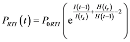 (2)
(2)
In the above equation, PPI (t) and PRTI (t) denote PI and RTI drug effectiveness at iteration number t, respectively. P0PI and P0RTI denote the initial value of PI and RTI drug effectiveness, respectively. V(t − 1), I(t − 1) and H(t − 1) denote the viral load, concentration on infected cells and the concentration of healthy cells at iteration number t − 1, respectively. V(ts), I(ts) and H(ts) denote viral load, concentration of infected cells and concentration of healthy cells at time of onset of treatment, respectively.
2.1.4. The Inputs and Outputs of Proposed Model
The RTI and PI antiretroviral drugs were considered as the inputs of our model. To consider these inputs, we used a parameter named effectiveness as PRTI and PPI for RTI and PI antiretroviral drugs, respectively [15] [29] . The time evolution of concentrations of normal healthy CD4+T cells, infected CD4+T cells (A1 + A2), CTLs, antibodies, dead cells and viral load, were considered as the outputs of our model. The curve of these variations has been drawn in the results section and each of them has been explained in detail.
2.2. Optimizing the Therapeutic Schedule by Applying Genetic Algorithms
After ensuring the validity of proposed CA model (according to the results obtained in Section 3.2), an optimal therapeutic schedule was presented by using Genetic Algorithms (GA). An introduction of GA can be found in [30] [31] . Since for HIV infected patients, long-term medication is prescribed, these patients suffer from side effects of antiretroviral drugs. Therefore, the most important advantage of using the obtained therapeutic schedule by GA is while maintaining the quality of the treatment, leading to a reduction in both drug dosage and the side effects of antiretroviral drugs. As we mentioned before, in order to prevent the patients from occurrence of drug-resistant, most of physicians prefer to apply cART method for HIV infected patients [32] . Also, as we will prove in section3.1, the use of cART method with maximal drug effectiveness, leading to better results (i.e. higher level of the steady state concentrations of healthy CD4+T cells, lower level of the steady state concentrations of infected CD4+T cells, as well as, lower level of viral load at steady state). For these reasons, the cART method with maximum drug effectiveness was used in our proposed therapeutic schedule. In presenting the optimal therapeutic schedule, in order to simply the simulations, we assumed that antiretroviral drugs (both RTI & PI drugs) are administered or interrupted weekly.
In GA, each of the therapeutic schedules was defined by a chromosome with m bits, that m defines the number of weeks of therapeutic schedule [33] . In this study, we assumed that each of therapeutic schedules contains a period of 32 weeks (i.e. weeks in 8 months) and the treatment was started at 160th week. A chromosome is a 2-state variable. Therefore, for each of weeks (bits) of therapeutic schedules (chromosomes), following modes may occur:
a) If the ith bit of a chromosome is set equal to zero, then it means that during the ith week of therapeutic schedule, no treatment is applied.
b) If the ith bit of a chromosome is set equal to one, then it means that during the ith week of therapeutic schedule, cART method with maximum drug effectiveness is applied.
Therefore, one of the values 0 or 1, was assigned randomly to each of bits of chromosome. Then, corresponding to the assigned value, the values of drug effectiveness were adjusted in CA model. Accordingly, if the assigned value was equal to zero, then in CA model, the values of both P0RTI and P0PI was set equal to zero (i.e. P0RTI = P0PI = 0). And if the assigned value was equal to one, then in CA model, the values of both P0RTI and P0PI was set equal to 0.9 (i.e. P0RTI = P0PI = 0.9).
In the GA optimization, the population size was set equal to 32 × 10 = 320. The reason of this choice was that each of chromosomes has 32 bits, and 10 different states can be assigned to each of bits. Therefore, with setting the population size equal to 320, many different therapeutic schedules will be evaluated by GA and obtained optimal therapeutic schedule will be more reliable. The GA optimization procedure ran on 50 generations. The operations and parameters of genetic algorithms that were applied in our simulations are shown in Table 2.
Table 2. The operators and parameters used for GA optimization.
The drug dosage and concentrations of healthy CD4+T cells and viral load at steady state due to applying a therapeutic schedule are the most important factors in evaluating the quality of that therapeutic schedule. Therefore, in order to evaluate the quality of each of chromosomes (therapeutic schedules), the following functions were calculated for each of chromosomes [33] .
 (3)
(3)
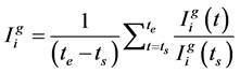 (4)
(4)
 (5)
(5)
In the above equations, ts indicates the time of onset of treatment; te indicates the time of end of treatment. ,
,  and
and  indicate the concentrations of healthy cells, viral load and drug dosage, respectively, that obtained from applying the therapeutic schedule related to ith chromosome of jth generation. Then for ith chromosome of jth generation, the following cost function was defined:
 (6)
(6)
A desirable therapeutic schedule is a schedule that by applying it, with minimum drug dosage, the concentration of healthy CD4+T cells and viral load at steady state reaches to maximum and minimum level, respectively. Considering this description and according to functions described above, that is more worthy chromosome for which the calculated value of the cost function is smaller (i.e.
 . Then the fitness function for ith chromosome of jth generation
  was defined as inverse of cost function:
 (7)
(7)
Since the fitness function is defined as the inverse of cost function, therefore, the highest calculated value of cost function is related to the fittest chromosome. According to GA optimization procedure, all of the chromosomes of first generation are sorted according to the value of cost function that was calculated for each of them. Chromosomes with smaller calculated value of cost functions were transferred to the next generation as the fittest chromosomes of first generation.
3. Simulation Results and Discussion
3.1. Results Obtained from Simulating the Proposed CA Model
In order to simulate the proposed CA model, a cell grid with size of 250 × 250 was considered. According to the defined initial numbers for each type of cells, an initial numbers of normal healthy cells, infected cells (A1), infectious viruses, CTLs and antibodies were distributed randomly in the grid space. According to the defined rules in Section 2.1.1 and with considering the values of Table 1 for parameters, we simulated the model for 600 iterations (each of iterations was considered as one week). The simulation was run 20 times with 20 different random initial configurations. Then the average of results obtained from 20 times run the simulation was shown for each of iterations. First we assumed that any types of antiretroviral drugs are not used. For this purpose, the values of parameters PRTI and PPI were considered as zero. Figure 4 shows the results obtained from this simulation.
For validating the results obtained from proposed model, we compared our results with the standard reference AIDS curve which has been shown in Figure 2. As this Figure 4 shows, the results obtained from our model are qualitatively in a good agreement with the reference curve. In the progress of AIDS, the concentrations of healthy and infected cells are of special importance. As long as the concentrations of healthy cells are higher than the threshold of AIDS (i.e. 20% of maximum number of healthy cells before infection occurs), the risk of death not threaten the patient. Therefore, from now on only the concentrations of healthy and infected cells will be investigated.
In the next step, we studied the effects of applying medication on the concentrations of healthy and infected cells. As we mentioned before, due to occurrence of drug-resistance and as a result of HIV mutation phenomenon, combined antiretroviral therapy (cART) method (the therapy method in which a combination of both of RTI and PI drugs is used) will be more effective in control of progression of AIDS. Therefore, in this study, the effects of applying cART method, with consideration of different values for drug effectiveness, are studied. The concentrations of healthy CD4+T cells and infected CD4+T cells (A1 + A2)

Figure 4. Simulation results obtained from proposed CA model during 48 weeks after initial infection (Here we have not considered any antiretroviral treatment in model).
obtained from simulating our CA model have been shown in Figure 5 and Figure 6, respectively. In our simulations, following conditions have been consi- dered: at first, we did not apply any medication and we called this situation as “without treatment”, then we considered applying cART method with minimum drug effectiveness (P0RTI = P0PI = 0.5), medium drug effectiveness (P0RTI = P0PI = 0.7) and maximum drug effectiveness (P0RTI = P0PI = 0.9). It should be noted that in all these conditions the treatment has been started from 160th weeks. In order to normalize the obtained results, the following measures were taken: a) in Figure 5, the average number of healthy cells at each of iterations, divided into the initial number of healthy cells. b) in Figure 6, the average number of infected cells at each of iterations, divided into the initial number of healthy cells to determine what fraction of normal healthy cells have became infected cells.
As Figure 5 shows, in terms of without treatment, the concentration of healthy cells will decline below the threshold of AIDS after about 250 weeks. While, in terms of applying cART, the concentration of healthy cells at steady state, remain in higher level than the threshold of AIDS. Also, we can see from this figure that the greater drug effectiveness causes more increase in the level of concentration of healthy cells at steady state. When we considered minimum, medium and maximum drug effectiveness, in compare with the case in which no treatment method was considered, the concentration of healthy cells at steady state has been increased 28%, 46% and 53%, respectively.

Figure 5. Fractions of concentrations of healthy CD4+T cells (H + HR) over weeks in presence of cART with different values of drug effectiveness. From up to down, the curves are related to applying cART with maximum drug effectiveness (P0RTI = P0PI = 0.9), cART with medium drug effectiveness (P0RTI = P0PI = 0.7), cART with minimum drug effectiveness (P0RTI = P0PI = 0.5) and no treatment, respectively. The treatment has been started from 160th week.
As Figure 6 shows, applying cART method causes a significant reduction in the level of infected cells at steady state. When we applied the cART method with minimum, medium and maximum drug effectiveness, in compare with condition in which no therapy method has been applied, the level of infected cells have been decreased 24%, 37% and 41%, respectively.
Since the viral load plays an important role in spread of infection, the level of infectious HIV particles was studied under following conditions: a) without treatment, b) with applying cART method with minimum, medium and maximum drug effectiveness. Figure 7 shows the level of load under conditions mentioned above. As this figure shows, by applying cART method with minimum, medium and maximum drug effectiveness in compare with the case of “no treatment”, the level of viral at steady state was reduced 55%, 65% and 69%, respectively. Thus, the best result (i.e. the lowest level of infectious viral load) obtained in presence of combined antiretroviral therapy with maximum drug effectiveness. Therefore, Comparing the results obtained in case of “without treatment” with other conditions in which a therapy method has been used shows that antiretroviral drugs, in addition to increasing the concentration of healthy cells, is leading to a reduction in the level of infectious viral load in the patient’s peripheral blood.
3.2. Validating the Obtained Results from CA Model through Comparing with Clinical Data
Clinical data collection in the field of AIDS is not a simple task. Gonzalez et al.,

Figure 6. Fractions of concentrations of infected CD4+T cells (A1+A2) over weeks in presence of cART with different values of drug effectiveness. From up to down, the curves are related to applying no treatment, cART with minimum drug effectiveness (P0RTI = P0PI = 0.5), cART with medium drug effectiveness (P0RTI = P0PI = 0.7) and cART with maximum drug effectiveness (P0RTI = P0PI = 0.9), respectively. The treatment has been started from 160th week.

Figure 7. Number of infectious viral load over weeks in presence of cART with different values of drug effectiveness. From up to down, the curves are related to applying no treatment, cART with minimum drug effectiveness (P0RTI = P0PI = 0.5), cART with medium drug effectiveness (P0RTI = P0PI = 0.7) and cART with maximum drug effectiveness (P0RTI = P0PI = 0.9), respectively. The treatment has been started from 160th week.
compared the results obtained from their CA model with clinical data which had been published in some of the authentic articles [15] . So in present work in order to validation of the results obtained from proposed CA model, we also apply the clinical data that had been used by Gonzales et al. In [35] nine patients were selected and were treated by applying cART. Treatment was started for these patients when the concentration of healthy CD4+T cells in their peripheral blood reached to 25% of concentration of this kind of cells in uninfected individual’s blood. These patients were followed over a period of eight months. The concentration of healthy CD4+T cells per microliter of patient’s peripheral blood was measured three times: once, right at the time of onset of treatment, second time, three weeks after onset of treatment and third time, eight months (24 weeks) after onset of treatment. In this reference, the average number of healthy CD4+T cells per microliter of an uninfected individual’s peripheral blood has been reported 970 ± 250 cells. In order to unify the scale of clinical data and results obtained from CA model, the clinical data were normalized by dividing them to average concentration of healthy CD4+T cells per microliter of an uninfected individual’s blood that has been reported in this reference. Figure 8(a) shows data relating to each of these patients. In order to comply with the conditions under which clinical data were recorded, we considered following assumptions: 1) In our model also, the treatment was started when the concentration of healthy CD4+T cells reached to 25% of initial concentration of this kind of cells. This

 (a)
(a) (b)
(b)
Figure 8. Comparing the clinical data of patients, with results obtained from CA model in presence of cART method using different values of effectiveness of drugs (P0RTI = P0PI = 0.5 & 0.9). Panel (a) circles depict concentrations of healthy CD4+T cells from nine patients who are treated with cART. These data have been collected at time of onset of treatment, 3 weeks and 24 weeks after initiation of treatment, respectively. Triangles depict the average values obtained for every week. These data are reported in Table 2 of [32] . Panel (b) depicts the fraction of concentrations of healthy CD4+T cells obtained from CA model by applying cART method for every week. Red and green bars depict results of CA model using minimum and maximum effectiveness of drugs, respectively. Also, blue bars depict the average values of real clinical data which are divided by the average of healthy CD4+T cells concentration in blood from non-infected individuals (970 ± 250 cells/µl).
happened at 220th week. 2) The simulations were ran nine times (to show nine patients) and at each time, the cART was started at 220th week. During a period of 24 weeks, every three weeks, the concentration of healthy CD4+T cells obtained from our model was recorded. 3) This procedure was done once with consideration of minimum and once again with maximum drug effectiveness. Figure 8(b) shows the comparison between the average of results obtained from our model and average of values obtained from clinical data. As can be observed in Figure 8(b), the highest compliance of clinical data with results obtained from proposed CA model arises when the drug effectiveness (P0RTI & P0PI) are considered minimal.
In [36] , ten patients were selected and were treated by cART method. These patents were followed over a period of 168 day (24 weeks). The viral load per milliliter of patient’s peripheral blood was measured at following times: right at time of onset of treatment and respectively, 21 days (3 weeks) and 168 days (24 weeks) after onset of treatment. Figure 9(a) shows the recorded clinical data for each of 10 patients with an average of them at each measured time interval. In order to compare results obtained from our model with clinical data, following factors were considered in our model: 1) the simulation was ran 10 times (to show 10 patients) and at each time the cART therapy was started at 160th week. 2) The concentrations of viral load obtained from CA model were recorded at same time intervals in which clinical data were measured. 3) This procedure was repeated once with minimum and once again with maximum drug effectiveness. Figure 9(b) shows the average of results obtained from our model in compare with real data. In order to unify the scale of clinical data and results obtained from CA model, we normalized both results and clinical data by dividing them to their values at the beginning of treatment. Therefore, we can show that the viral load at every week is what fraction of its value at the beginning of treatment. As both Figure 9(a) and Figure 9(b) show, clinical data, as well as results obtained from our CA model, reflect this fact that due to use of cART method the viral load is declined sharply about 3 weeks after onset of treatment. This proves that cART method can inhibit the viral load in patient’s peripheral blood quickly and successfully. As Figure 9(b) shows, the highest compliance of clinical data with our results arises when the drug effectiveness (P0RTI & P0PI) are considered maximal.
3.3. Results Obtained from GA Optimization
All steps of GA optimization were repeated for 50 generations. Figure 10(a) and Figure 10(b) show the average cost function and fitness function over generations, respectively. As Figure 10(a) shows, during the GA optimization over generations, the average cost function is decreasing and according to the inverse relation between cost function and fitness function, as Figure 10(b) shows, the average fitness function is increasing. Reduction in cost function and increase in fitness function during generation, are related to optimization of therapeutic schedule and leading to obtain the optimal schedule. In the last generation, the chromosome with smallest (biggest) value of cost function (fitness function) was presented as the best chromosome. Therefore, by applying the therapeutic schedule related to fittest chromosome, the highest concentration of CD4+T cells, as well as, the lowest viral load at steady state and simultaneously the lowest drug dosage will be obtained. Figure 11 shows the optimal therapeutic schedule obtained from GA optimization.
 (a)
(a) (b)
(b)
Figure 9. Panel (a) Circles depict number of copies of HIV-RNA/ml in blood of 10 patients who are treated with cART. These data are collected at the time of onset of treatment, 3 weeks and 24 weeks after initiation of treatment. Squares depict the average values obtained for every week. These data are reported in [36] . Panel (b) shows the average results obtained from CA model by applying cART with different values of drug effectiveness, for every week. Obtained values are divided to amount of viral load at time of start of treatment. Red and green bars are related to applying minimum and maximum drug effectiveness, respectively. Blue bars depict average of viral load obtained from clinical data which are divided to average of viral load at time of onset of treatment.
3.4. Validating the Results Obtained from GA Optimization
In order to prove desirable performance of optimal therapeutic schedule obtained from GA optimization, three different therapeutic schedules were defined and results obtained from applying these schedules were compared with each other. These therapeutic schedules are as below. In each of the therapeutic schedules the treatment was started from 160th week.
 (a)
(a) (b)
(b)
Figure 10. Panel (a) depicts the average of cost functions calculated for all chromosomes related to each of generations. Panel (b) is related to average fitness function over generations during GA optimization.
a) Full therapy with maximum drug dosage: in this case the cART with maximum drug dosage (i.e. PPI = PRTI = 0.9) was applied at every week.
b) Best therapy with optimal drug dosage: in this case the optimal therapeutic schedule obtained from GA optimization was applied.
c) Random therapy: in this case, the number of weeks in which cART with minimum drug dosage is applied, was set equal to the number of therapy weeks in the case of best therapy, but a random therapeutic schedule was applied during these weeks.

Figure 11. This figure depicts the value of drug effectiveness at each of the weeks related to optimum therapeutic schedule obtained from GA optimization. The cART therapeutic method has been started from 160th week.
Figure 12 shows a comparison between levels of drug dosage, as well as, the concentrations of healthy and infected CD4+T cells at steady state resulting from applying these three therapeutic schedules.
As Figure 12 shows, the steady state concentration of healthy CD4+T cells (infected CD4+T cells) obtained from “Best therapy” is just 3.9% (2%) lower (higher) than the steady state concentrations of these cells obtained from “Full therapy”. Also, the level of drug dosage in “Best therapy” is 47% lower than the level of drug dosage in “Full therapy”. Therefore, the steady state concentration of healthy and infected CD4+T cells obtained from “Best therapy” is very close to the steady state concentrations of these cells obtained from “Full therapy”, while, the drug dosage obtained from applying “Best therapy”, in compare with applying “Full therapy”, is decreased significantly. By comparing results obtained from optimum therapy schedule and results obtained from random therapy schedule we find that by applying random therapeutic schedule, although the level of drug dosage is identical with the case in which optimum therapy schedule has been applied, the steady state concentration of healthy (infected) CD4+T cells is 12.9% (9.4%) lower (higher) than the steady state concentrations of these cells obtained from optimum therapy.
Therefore, by concluding our results we find that by applying full therapy schedule, although the quality of treatment is maintained, due to the high level of drug dosage, the patient will suffer from side effects of antiretroviral drugs. On the other hand, by applying random therapy schedule, although the level of drug dosage has been decreased, the quality of treatment also decreased. But by

Figure 12. Drug dosage and concentrations of healthy and infected cells obtained from applying three different therapeutic methods. The set of three bars located on the left, middle and right of the figure, are related to applying full therapy method, best therapy method and random therapy method, respectively. Blue bars and red bars depict the fractions of steady state concentrations of healthy and infected cells, respectively. The green bars are related to the fractions of total drug dosage obtained from each of therapeutic method.
applying optimal therapy schedule that obtained from GA optimization, while maintaining the quality of treatment, leading to reduction in both, level of drug dosage and the side effects of antiretroviral drugs.
4. Conclusions
In this study, by using genetic algorithms (GA), we found an optimum therapeutic schedule for HIV infected patients based on combined antiretroviral therapy (cART) method. In order to simulate the effects of therapy, two-dimen- sional cellular automata (CA) model was used. This CA model depicts the dynamics involved in the interactions between acquired immune system and HIV, in the peripheral blood of HIV infected individuals. This model was developed taking into account the following points: a) occurrence of mutation phenomena, b) existing time delay in the immune system, c) the role of latently infected cells in spread of infection, d) the effects of antiretroviral drugs such as reverse transcriptase inhibitors (RTI) and protease inhibitors (PI), e) occurrence of drug resistance in patients who are under antiretroviral therapy.
For this purpose, first, we collected appropriate rules related to HIV infection in patient’s peripheral blood according to reference articles and base on expert knowledge including books and medical journals in the field of AIDS and we developed our CA model using these rules. At this step, by comparing the results obtained from our CA model with reference HIV curve, we showed that our results are in a good agreement with the existing reality in the interactions between acquired immune system and HIV. At next step, we studied the effects of cART by adding some new states and parameters to the proposed CA model. For this purpose, we considered a parameter named drug effectiveness for each of RTI and PI drugs that were shown by PRTI and PPI, respectively. Occurrence of drug resistance was considered by a negative exponential equation. The concentrations of healthy and infected CD4+T cells over the weeks and the level of viral load were obtained by consideration of different values for PRTI and PPI. Our results showed that by applying maximum effectiveness of RTI and PI drugs, compared with cases in which no treatment was applied, the steady state concentrations of healthy (infected) CD4+T cells were increased (decreased) 53% (41%). Also, the use of cART with maximum drug effectiveness led to a 69% reduction in the steady state level of viral load. In order to validate the results obtained from our proposed CA model in the cases in which cART was applied, we used clinical data which are provided in authoritative articles. By comparing results obtained from our model with clinical data, we prove that the best compliance between our results and clinical data arises when we consider minimum effectiveness for antiretroviral drugs.
In the second phase of this study, we used GA optimization to provide an optimal therapeutic schedule of cART with maximum drug effectiveness based on structured interruptions. To prove the effectiveness of obtained therapeutic schedule from GA optimization, three different therapy schedules were defined as following: a) Full therapy, b) Best therapy with optimum drug dosage, c) Random therapy. According to each of these therapy schedules, cART with minimum drug effectiveness was applied or interrupted at each of weeks in the proposed CA model. Then the steady state concentrations of healthy and infected CD4+T cells, and the amount of drug dosage obtained from applying each of these schedules were presented as our results. Our results showed that by applying the optimum therapeutic schedule obtained from GA optimization, the quality of treatment (i.e. high steady state concentration of healthy cells and low steady state concentration on infected cells) is very close when the full therapy schedule was applied. But the main point is that applying the optimum therapeutic schedule, compared with full therapy schedule, led to 47% reduction in the amount of drug dosage. Therefore, the optimum therapeutic schedule provides the high quality treatment, low amount of drug dosage and low side effects of antiretroviral drugs, simultaneously.
The CA model that was developed for AIDS in this study, involves the biological facts of this disease and it could depict all three patterns of progression of HIV infection properly. Most importantly, the effects of applying different antiretroviral drugs were also considered in this model. Therefore, as an application of the model developed in this study can be said, by using this model, physicians can evaluate the effects of applying different therapeutic methods on virtual patients through model, without requiring costly clinical trials on real patients. Also, by using Genetic Algorithms (GA), the best therapeutic schedule that provides the high quality treatment with low amount of drug dosage, can be obtained through this model. Therefore, results obtained from this model can be useful for physicians. However, this model is still developing. Finding newer and more accurate rules, more accurate estimating of model parameters, adding new states to show different aspects of disease, investigating more varied therapeutic methods and adjusting the drug dosage in the therapeutic schedule can be considered as future works.
Cite this paper
Golpayegani, G.N., Jafari, A.H. and Dabanloo, N.J. (2017) Providing a Therapeutic Scheduling for HIV Infected Individuals with Genetic Algorithms Using a Cellular Automata Model of HIV Infection in the Peripheral Blood Stream. J. Biomedical Science and Engineering, 10, 77-106. https://doi.org/10.4236/jbise.2017.103008
References
- 1. Weiss, R. (1993) How Does HIV Causes AIDS? Science, 260, 1273-1279.
https://doi.org/10.1126/science.8493571 - 2. AIDS Epidemic Update, World Health Organization (WHO), 2011.
- 3. Craig, I. and Xia, X. (2005) Can HIV/AIDS Be Controlled? Applying Control Engineering Concepts outside Traditional Fields. IEEE Control System Magazine, 25, 80-83.
https://doi.org/10.1109/MCS.2005.1388805 - 4. Imamichi and Tomozumi (2004) Action of Anti-HIV Drugs and Resistance: Reverse Transcriptase Inhibitors and Protease Inhibitors. Current Pharmaceutical Design, 10, 4039-4053.
- 5. Teklay, G., Legesse, B. and Legesse, M. (2013) Adverse Effects and Regimen Switch among Patients on Antiretroviral Treatment in a Resource Limited Setting in Ethiopia. Pharmacovigilance, 1.
https://doi.org/10.4172/2329-6887.1000115 - 6. Isham, V. (1989) Mathematical Modeling of the Transmission Dynamics of HIV Infection and AIDS. Mathematical and Computer Modeling, 12, 1187.
https://doi.org/10.1016/0895-7177(89)90269-0 - 7. Wodarz, D. and Nowak, M.A. (2000) Mathematical Models of HIV Pathogenesis and Treatment. BioEssays, 24, 1178-1187.
https://doi.org/10.1002/bies.10196 - 8. Landi, A., Mazzoldi, A., Andreoni, C., Bianchi, M., Cavallini, A., Laurino, M., Ricotti, L., Iuliani, R., Matteoli, B. and Ceccherini, L. (2008) Modeling and Control of HIV Dynamics. Computer Methods and Program in Biomedicine, 89, 62-68.
https://doi.org/10.1016/j.cmpb.2007.08.003 - 9. Perrin, D., Ruskin, H.J. and Crane, M. (2008) An Agent-Based Approach to Immune Modeling: Priming Individual Response. World Academy of Science, Engineering and Technology, 2, 167-173.
- 10. Gutowitz, H. (1991) Cellular Automata: Theory and Experiment. MIT Press, Cambridge, MA.
- 11. Xiao, X., Shao, S. and Chou, K. (2006) A Probability Cellular Automaton Model for Hepatitis B Viral Infection. Biochemical and Biophysical Research Communications, 342, 605-610.
https://doi.org/10.1016/j.bbrc.2006.01.166 - 12. Dos Santos, R.M.Z. (2001) Dynamics of HIV Infection: A Cellular Automata Approach. Physical Review Letters, 87, 1-4.
- 13. Sloot, P., Chen, F. and Boucher, C. (2002) Cellular Automata Model of Drug Therapy for HIV Infection. Lecture Notes in Computer Science, 2493, 282-293.
https://doi.org/10.1007/3-540-45830-1_27 - 14. Shi, V., Tridane, A. and Kuang, Y. (2008) A Viral Load-Based Cellular Automata Approach to Modeling HIV Dynamics and Drug Treatment. Journal of Theoretical Biology, 253, 24-35.
https://doi.org/10.1016/j.jtbi.2007.11.005 - 15. Gonzalez, R.E.R., Coutinho, S., Dos Santos, R.M.Z. and Figueiredo, P.H. (2013) Dynamics of HIV Infection under Antiretroviral Therapy: A Cellular Automata Approach. Physica A: Statistical Mechanics and Its Applications, 392, 4701-4716.
https://doi.org/10.1016/j.physa.2013.05.056 - 16. Gonzalez, R.E.R., Figueiredo, P.H. and Coutinho, S. (2012) Cellular Automata Approach for the Dynamics of HIV Infection under Antiretroviral Therapies: The Role of Virus Diffusion. Physica A: Statistical Mechanics and Its Applications, 392, 4717- 4725.
https://doi.org/10.1016/j.physa.2012.10.036 - 17. Jafelice, R.M., Bechara, B.F.Z., Barros, L.C., Bassanezi, R.C. and Gomide, F. (2009) Cellular Automata with Fuzzy Parameters in Microscopic Study of Positive HIV Individuals. Mathematical and Computer Modeling, 50, 32-44.
https://doi.org/10.1016/j.mcm.2009.01.008 - 18. Mostafa, K., Khalid, H. and Noura, Y. (2014) Modeling the Adaptive Immune Response in Hiv Infection Using a Cellular Automata. International Journal of Engineering and Computer Science, 3, 5040-5045.
- 19. Rowland-Jones, S., Pinheiro, S., Kaul, R., Hansasuta, P., Gillespie, G., Dong, T., et al. (2001) How Important Is the “Quality” of the Cytotoxic T Lymphocyte (CTL) Response in Protection against HIV Infection? Immunology Letters, 79, 15-20.
https://doi.org/10.1016/S0165-2478(01)00261-9 - 20. Yang, O., Sarkis, P., Ali, A., Harlow, J., Brander, C., Kalams, S., et al. (2003) Determinants of HIV-1 Mutational Escape from Cytotoxic T Lymphocytes. The Journal of Experimental Medicine, 197, 1365-1375.
https://doi.org/10.1084/jem.20022138 - 21. Connick, E., Marr, D.G., Zhang, X.Q., Clark, S.J., Saag, M.S., Schooley, R.T., et al. (2009) HIV-Specific Cellular and Humoral Immune Response in Primary HIV Infection. AIDS Research and Human Retroviruses, 12, 1129-1140.
https://doi.org/10.1089/aid.1996.12.1129 - 22. Loscalzo, J., Kasper, D., Jameson, J., Hauser, S., Fauci, A. and Longo, D. (2015) Harrison’s Principal of Internal Medicine—Infectious Diseases Part. 19th Edition, McGraw-Hill, New York.
- 23. Alcamo, I.E. (2003) AIDS: The Biological Basis. 3rd Edition, Jones and Bartlett Publishers, London.
- 24. McCune, J.M. (2001) The Dynamics of CD4+T-Cell Depletion in HIV Disease. Nature, 410, 974-979.
https://doi.org/10.1038/35073648 - 25. Tassie, J.M., Grabar, S., Lancar, R., Deloumeaux, J., Bentata, M. and Costagliola, D. (2002) Time to AIDS from 1992 to 1999 in HIV-1 Infected Subjects with Known Date of Infection. Journal of Acquired Immune Deficiency Syndromes, 30, 81-87.
https://doi.org/10.1097/00042560-200205010-00011 - 26. Althaus, C.L. and De Boer, R.J. (2011) Implications of CTL-Mediated Killing of HIV-Infected Cells during the Non-Productive Stage of Infection. PLoS ONE, 6, e16468.
https://doi.org/10.1371/journal.pone.0016468 - 27. Pat Bucy, R. (2004) Viral and Cellular Dynamics in HIV Disease. Current HIV/ AIDS Reports, 1, 41-46.
- 28. Caetano Marco, L.A., de Souza Jam, F. and Yoneyama, T. (2008) Optimal Medication in HIV Seropositive Patient Treatment Using Fuzzy Cost Function. American Control Conference, Seattle, 11-13 June 2008, 2227-2232.
- 29. Xia, X. (2007) Modelling of HIV Infection: Vaccine Readiness, Drug Effectiveness and Therapeutical Failures. Journal of Process Control, 17, 253-260.
https://doi.org/10.1016/j.jprocont.2006.10.007 - 30. Charbonneau, P. (2002) An Introduction to Genetic Algorithms for Numerical Optimization. NCAR Technical Note, Boulder, Colorado.
- 31. Roeva, O. (2005) Genetic Algorithms for a Parameter Estimation of a Fermentation Process Model: A Comparison. Bioautomation, 3, 19-28.
- 32. Autran, B., Carcelain, G., Li, T.S., Blanc, C., Mathez, D. and Tubiana, R. (1997) Positive Effects of Combined Antiretroviral Therapy on CD4+T Cell Homeostasis and Function in Advanced HIV Disease. Science, 277, 112-116.
https://doi.org/10.1126/science.277.5322.112 - 33. Castiglione, F., Pappalardo, F., Bernaschi, M. and Motta, S. (2007) Optimization of HAART with Genetic Algorithms and Agent-Based Models of HIV Infection. Bioinformatics, 23, 3350-3355.
https://doi.org/10.1093/bioinformatics/btm408 - 34. Goldberg, D.E. and Deb, K. (1991) A Comparative Analysis of Selection Schemes Used in Genetic Algorithms. In: Rawlins, G., Ed., Foundations of Genetic Algorithms, Morgan Kaufmann Publishers, San Mateo, CA, 69-93.
- 35. Zhang, Z., Notermans, D.W., Sedgewick, G., Cavert, W., Wietgrefe, S., Zupancic, M., et al. (1998) Kinetics of CD4+T Cell Repopulation of Lymphoid Tissues after Treatment of HIV-1 Infection. PNAS, 95, 1154-1159.
https://doi.org/10.1073/pnas.95.3.1154 - 36. Notermans, D.W., Staskus, K., Wietgrefe, S.W. and Zupancic, M. (1997) Kinetics of Response in Lymphoid Tissues to Antiretroviral Therapy of HIV-1 Infection. Science, 276, 960-964.
https://doi.org/10.1126/science.276.5314.960 - 37. Ruffault, A., Michelet, C., Jacquelinet, C., Guist’au, O., Genetet, N., Bariou, C., Colimon, R. and Cartier, F. (1995) The Prognostic Value of Plasma Viremia in HIV- Infected Patients under AZT Treatment: A Two-Year Follow-Up Study. Journal of Acquired Immune Deficiency Syndromes and Human Retrovirology, 9, 243-248.
https://doi.org/10.1097/00042560-199507000-00004 - 38. Adams, B.M., Banks, H.T., Davidian, M., Kwon, H., Tran, H.T., Wynne, S.N., et al. (2005) HIV Dynamics: Modeling, Data Analysis, and Optimal Treatment Protocols. Journal of Computational and Applied Mathematics, 18, 10-49.
https://doi.org/10.1016/j.cam.2005.02.004 - 39. Pappalardo, F., Mastriani, E., Lollini, P.L. and Motta, S. (2006) Genetic Algorithm against Cancer. Lectures Notes in Computer Science, 3849, 223-228.
https://doi.org/10.1007/11676935_27
Abbreviation Note List
HIV: Human Immunodeficiency Virus
AIDS: Acquired Immunodeficiency Syndrome
RTI: Reverse Transcriptase Inhibitors
PI: Protease Inhibitors
cART: Combined Antiretroviral Therapy
CA: Cellular Automata
ODE: Ordinary Differential Equations
PDE: Partial Differential Equations
AB: Anti Bodies
GA: Genetic Algorithms