Journal of Biomedical Science and Engineering
Vol. 5 No. 11 (2012) , Article ID: 24667 , 20 pages DOI:10.4236/jbise.2012.511076
Efficient hemodynamic states stimulation using fNIRS data with the extended Kalman filter and bifurcation analysis of balloon model
![]()
1Electrical Engineering Department, École Polytechnique de Montréal, Montreal, Canada
2Wellman Center for Photomedicine, The Harvard-MIT Health Sciences and Technology, Harvard Medical School, Cambridge, USA
Email: ehsan.kamrani@ieee.org
Received 2 July 2012; revised 6 August 2012; accepted 30 August 2012
Keywords: BOLD Signal; fNIRS; Brain Monitoring; Kalman Filter; Stability; Simulation and Modeling
ABSTRACT
This paper introduces a stochastic hemodynamic system to describe the brain neural activity based on the balloon model. A continuous-discrete extended Kalman filter is used to estimate the nonlinear model states. The stability, controllability and observability of the proposed model are described based on the simulation and measurement data analysis. The observability and controllability characteristics are introduced as significant factors to validate the preference of different hemodynamic factors to be considered for diagnosis and monitoring in clinical applications. This model also can be efficiently applied in any monitoring and control platform include brain and for study of hemodynamics in brain imaging modalities such as pulse oximetry and functional near infrared spectroscopy. The work is on progress to extend the proposed model to cover more hemodynamic and neural brain signals for real-time in-vivo application.
1. INTRODUCTION
Brain function can be studied by monitoring two major types of signals: neuronal signal and hemodynamic signal. Investigating functional principles of the human brain requires a multimodal approach. The most widely used imaging techniques are functional magnetic resonance imaging (fMRI) and functional near infra-red spectroscopy (fNIRS). They rely on an indirect signal, the blood oxygenation level-dependent (BOLD) contrast [1], which is caused by an increase in oxygen delivery, strongly exceeding the metabolic demand [2]. fNIRS is the only neuroimaging system capable of detecting both fast neuronal signal and slow hemodynamic signal [3]. The other brain monitoring methods such as electro encephalogram (EEG) and magneto encephalogram (MEG) can only measure the fast neuronal signal (electrophysiological aspect), the positron emission tomography (PET) and fMRI can measure only the slow hemodynamic signal (metabolic aspect). fNIRS obtains information on cerebral oxygenation, blood flow, activation, blood volume and metabolic status of the brain, not otherwise obtained with any single method and at a remarkably low cost.
In fNIRS, the brain tissue is penetrated by near-infrared (NIR) radiation and the backscattered signal is observed to investigate the brain’s function. In NIR range (650 nm - 950 nm), water has relatively low absorption while oxyand deoxy-hemoglobin have high absorption. Due to these properties, NIR light can penetrate biological tissues in the range of 0.5 - 3 cm allowing investigation of relatively deep brain tissues, and ability to differentiate between healthy and diseased tissues [4].
However the mapping between NIRS signals and the underlying variables is not straightforward, as a number of different causes may give rise to the same signal changes. Thus in order to correctly interpret and maximize the clinical usefulness of the information that can be extracted from NIRS data, a model of the underlying physiology is required [3]. The highly dependency and correlation of neurons processing, metabolic and vascular responses are conceptually well known in time and state space [5], but still the details on the translation between an ensemble of neurons firing and the ensuing increase in focal cerebral blood flow is a controversial issue. The most popular model to describe the neural activity according to the data from fMRI, is balloon model, which relates BOLD signal to the blood flow. This model is a nonlinear hemodynamic model and the measurements usually have a noisy behavior. Furthermore, the electromagnetic field produced by neurons is very weak and noisy, so the signal-to-noise-ratio (SNR) is very low.
We have used a Kalman filter as a statistical method to extract data from the signal and increase the SNR. In order to use Kalman filter we should have a model which represents the relation between neural activity (hemodynamic response) and the BOLD signal. Here the balloon model is used. We have used NIRS data on a balloon-based model with a stochastic hemodynamic system model to describe noise. An extended Kalman filter is applied as a reasonable model to estimate the nonlinear model states and output of the balloon model.
Since neuronal activity induces this hemodynamic response, the BOLD signal provides a noninvasive measure of neuronal activity. Understanding the mechanisms that drive this BOLD response is fundamental for accurately inferring the underlying neuronal activity [4]. The goal of this study is to systematically predict spatiotemporal hemodynamics from a biophysical model, then test these using fNIRS study of the visual cortex. Using this theory, we predict and empirically confirm the existence of hemodynamic waves in cortex and validate them regarding to the stability, controllability and observability.
As a consequence, in this paper the general background of hemodynamic response and BOLD signal is explained in section 2 and the impact of stability is addressed. The proposed model is introduced in section 3. Section 4 presents the simulation and experimental results following by analysis and discussions on the stability, controllability and observability of the proposed system.
2. BOLD SIGNAL AND HEMODYNAMIC RESPONSE
2.1. BOLD Signal
In order to measure the neural activity of the brain the EEG and MEG could be applied for electrophysiological aspects and the MRI and PET for metabolic aspects. fMRI is one of the most popular methods of neuroimaging, which uses hemodynamic response to show the neural activity of the brain. When the blood oxygenation changes in the brain, it shows that we have a neural activity. So, this is a way to track the neural activity by detecting the hemodynamic changes in the brain. Hemodynamic is the study of blood flow in the circulatory system and fMRI detects these hemodynamic changes. When a neural activity occurs, neurons need glucose and oxygen from blood and according to this need, blood sends glucose to the neuron. This process is called hemodynamic response and leads to increase in oxyhemoglobin in the vein vessels and produces a detectable change for MRI which is called BOLD signal. This BOLD signal shows the brain activity and fMRI uses this signal to show this activity.
Among all the fMRI methods, BOLD contrast is the dominant technique. The BOLD signal is sensitive to the local deoxyhemoglobin concentration; however the BOLD signal does not directly measure the neural activity itself. Instead the BOLD effect is sensitive to a series of physiological responses that are referred collectively as the hemodynamic response for activation. Changes in neural activity engender complex changes in physiological states, including the cerebral blood flow (CBF), cerebral blood volume (CBV), and cerebral oxygen consumption rate (CMRO2), which in turn alters the local deoxyhemoglobin concentration. The most standard fMRI analysis methods use the General Linear Model (GLM), which assumes a linear relationship between the neural activity and the BOLD response. fNIRS is a non-invasive, minimally intrusive safe imaging system applied for long-term and bedside brain monitoring. Comparing to other brain imaging systems, fNIRS is the only neuroimaging system capable of detecting both fast neuronal signal and slow hemodynamic signal [6]. It allows determining the Δ[HbO], Δ[HbR] and Δ[HbT]. While offers a high temporal resolution, but it has a moderate spatial resolution (~1 cm concerning the topography of cortex).
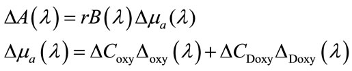
In fNIRS, the brain tissue is penetrated by near-infrared (NIR) radiation and the reflected signal is observed to investigate the brain’s function. In NIR range (650 nm - 950 nm), water has relatively low absorption while oxyand deoxy-hemoglobin have high absorption. Due to these properties, NIR light can penetrate biological tissues in the range of 0.5 - 3 cm allowing investigation of relatively deep brain tissues, and ability to differentiate between healthy and diseased tissues [7]. The light attenuation changes (ΔA) correlation to the changes in concentration (ΔC) of oxyand deoxyhemoglobin are calculated based on Beer-Lambert law as follow:
 (1)
(1)
where r is the source-detector separation distance and B is differential path-length factor implies the effect of scattering on attenuation. The main hypothesis that a homogenous change of absorption in the tissue under investigation, is violated by the fact that focal functional activation elicits focal changes in just one layer of the illuminated tissue of the cortex. This can cause some difficulties such as Cross talk, Extracerebral blood volume changes and Partial volume effect. To reach the brain the near-infrared light must transverse the scalp and skull. A blood volume change in extra-cerebral tissue will lead to an artefactual reconstruction of cerebral activation changes.
The partial volume effect is due to the mismatch between the volume sampled and the volume, actually activated NIRS underestimates the hemoglobin concentration changes. If the wavelength dependency of the differential path-length factor is not adequately determined, the Δ[oxy-Hb] can mimic Δ[HbR] and vice-versa. This phenomenon called cross-talk and can be minimized using optimal wavelength combinations, down to a few percentages. Considering the morphological information for the analysis of the NIRS data also will reduce the cross-talk [5]. BOLD signal has been applied in several studies to understand the human brain function [6-15]. Cognitive neuroscientists applying BOLD signal to an extent that the terms activation and deactivation of the human cortex are now broadly used to denote changes in T2 and T2* caused by the hemodynamic response. Current works undergoing to uncover the correlation between the BOLD signal and Δ[HbR] (or Δ[HbO]). The CBF variations also can be determined using arterial spin labelling (ASL).
There are a higher correlation between [HbT] and BOLD or a similar level of correlation of the BOLD signal to [HbR] and [HbO]. Mathematical and analytical models can be used to simulate the extraand intravascular contributions to BOLD-signal variations. These models are based on this fact that the extra-vascular effects on the BOLD signal depend on the field gradient around the vessel, which is mainly a function of [HbR]. Dependency on the total haemoglobin concentration (BOLD-CBV) and also on [HbR] (BOLD-deoxy), are the main components contributing to the global BOLD-signal variations [5].
2.2. Hemodynamic Response
The hemodynamic response function (HRF) is the BOLD response for a very short stimulus. In the GLM analysis, the BOLD response is modeled as a convolution of the neural activity with a HRF; however, the neural activities are usually approximated by the stimulus function rather than being directly measured. The shape of the HRF is often approximated by a single or sum of two Gamma functions. Deconvolving the fMRI response with the HRF is important in understanding the dynamics of the underlying neural activity [16,17]. However a large variation can be noticed across individual subjects in terms of HRFs and this variation can affect parameter estimation and detection of significant voxels.
However the validity of a linear framework analysis has been debatable and many studies have come to an agreement of the linear assumption on the interstimulus intervals (ISI) larger than a threshold. A threshold value of 2 - 3 s is agreed in [18] while the work presented in [17] agrees on a 4 - 6 s. Nevertheless, many experimental observations have provided evidence of the deviation of BOLD from linearity [19]. With these observations of nonlinearity of the BOLD response, several researchers have attempted to handle nonlinear characterization for these underlying brain processes. In [20], the linear model of heomodynamic response presented in [21] is extended to cover nonlinear responses using a Volterra series expansion. At the same time the first compelling model for heomodynamic signal transduction in fMRI was presented in [10], namely the Balloon Model. Several works have recently used this physiological model in the analysis of fMRI data, in the context of parameter estimation.
The work presented in [13] uses the Buxton-Fritson model, where the Buxton’s balloon model [22] is added with a damped oscillator to model the blood flow [2]. They used a local linearization transfer function in the Kalman filter methodology, allowing physiological noise in addition to the measurement noise. The work presented in [23] investigates the above physiological model plus the integrated version of the balloon model [24]. They use a maximum likelihood approach for the model based optimization of the parameter estimation, however only the measurement noise is dealt with the system modeling. Other than the state space linearized filter approaches, nonlinear filtering strategies have been applied for the estimation of the states and parameters from the BOLD responses. A particle filter approach is proposed in [25], while [26] applies an unscented Kalman filter (UKF) methodology for fMRI data analysis [16]. Models of the underlying hemodynamic and physiologic processes which give rise to the BOLD response have recently been incorporated into a more complete nonlinear system. The system can be considered as consisting of five subsystems linking: 1) neural activity to changes in flow; 2) changes in flow to oxygen delivery to tissue; 3) changes in flow to the changes in blood volume and venous outflow; 4) changes in flow, volume and oxygen extraction fraction to changes in deoxyhemoglobin, and finally; 5) changes in volume and deoxyhemoglobin to the BOLD response [9].
Hemodynamic responses to neuronal activity are observed experimentally in fMRI data via the BOLD signal, which provides a noninvasive measure of neuronal activity. Understanding the mechanisms that drive this BOLD response, combined with detailed characterization of its spatial and temporal properties, is fundamental for accurately inferring the underlying neuronal activity [10]. Such an understanding has clear benefits for many areas of neuroscience, particularly those concerned with detailed functional mapping of the cortex [6], those using multivariate classifiers that implicitly incorporate the spatial distribution of BOLD [7], and those that focus on understanding and modeling spatiotemporal cortical activity [13,14]. The temporal properties of the hemodynamic BOLD response have been well characterized by existing physiologically based models, such as the balloon model [15]. Although the spatial response of BOLD has been characterized experimentally via hemodynamic point spread functions [27], it is commonly agreed that the spatial and spatiotemporal properties are relatively poorly understood [28].
Developed biophysical model in [15] is motivated by Davis model but incorporates the oxygen limitation model and blood volume changes as integral parts. This model is based on the dynamic changes in Δ[HbR] during brain activation. The model incorporates the conflicting effects of dynamic changes in both blood oxygenation and blood volume. It shows distinct transients in the Δ[HbR] and the BOLD signal including initial dips and overshoots and a prolonged post-stimulus undershoot of the BOLD signal. The initial validation of this model comparing to the experimental measurements of flow and BOLD changes during a finger-tapping task shows reasonable agreement [15]. Both works presented at [15,28] are developed and validated only based on the experimental measurements acquired from MRI data on a specific region of the brain cortex and no specific application is proposed and validated based on the developed models. Despite the widespread use of functional neuroimaging techniques [13-16,22-32], the physiological changes in the brain that accompanying neural activation are still poorly understood [15-27,29].
Many studies work from the premise that the hemodynamic BOLD response is space-time separable, i.e. is the product of a temporal HRF and a simple Gaussian spatial kernel. Neglecting spatial effects such as voxelvoxel interactions and boundary conditions (e.g., blood outflow from one voxel must enter neighboring ones) ignores important phenomena and physical constraints that could be used to increase signal to noise ratios and to improve inferences of neural activity and its spatial structure.
Here we have presented a modified and integrated version of the balloon model, using state space system realization to be easily applied in any control system. We prefer to use this particular version of the balloon model since it has many degrees of freedom comparing to the other models [2,22] and can therefore produce a more desired behavior. Using this model one can analyze the fMRI data with robust nonlinear filtering techniques [16].
2.3. BOLD/Hemodynamic Stability
Every state requires pharmacologic or mechanical support to maintain a normal blood pressure or adequate cardiac output. The human body possesses a unique set of organs that are responsible for providing homeostatic balance to the body’s fluids. The kidneys regulate fluid and electrolyte balance in order to maintain the intracellular and extracellular fluid volumes and ion composition within tight limits. When kidneys fail to function normally, fluid is retained and several ions and solutes accumulate. The consequences may be life threatening. The major compensatory mechanisms include sympathetic nervous system activation of peripheral vasoconstriction together with modest heart rate acceleration to ensure the haemodynamic stability of the patient. Over the years, many monitoring tools have been developed in the hope of predicting intra-dialytic hypotensive episodes. Similarly many methods have been utilized to prevent dialysis induced complications: ultrafiltration and dialysate sodium profiling, varying ultrafiltration based on frequent BP measurements, etc. [32,33]. In the brain, realtime monitoring of hemodynamic states and preserve their stability provides a significant mechanism for fast and reliable brain monitoring especially in early detection of seizure and epilepsy or in brain-machine interaction studies.
3. PROPOSED MODEL
3.1. The Extended Balloon Model
The most popular biophysical model detailing different aspects of the hemodynamic response to describe the neural activity according to the data from fMRI and fNIRS is the balloon model which relates BOLD signal to the blood flow. Balloon model [22] is a Linear Model which an epileptic tip generates a localized hemodynamic response. It allows calculating normalized changes in the hemodynamic observables such as the CBV or [HbR]. It was initially based on the simplifying assumption of a venous balloon, an oxygen extractor and a trapezoidal change in CBF.
While this model is of supreme relevance to any multimodal assessment of the vascular response, it has been neglected by most of the combined fNIRS–fMRI experiments. The major assumption is that the venous balloon constitutes the only origin of the change in CBV and [HbR] generating the BOLD signal. The balloon model is expanded by a difference in normalized venous out-flow  and normalized arterial inflow
 . The CBF is also considered identical to
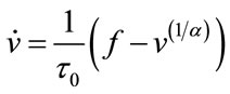
  in most works [4,5,8-10]. Conservation of mass then defines the change in the normalized blood volume v in the venous balloon as follow:
 (2)
(2)
here  is the mean transit time through the compartment,
  (0 - 30 s) indicated the viscoelastic time constant (inflation) and
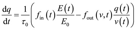
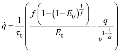
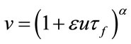
  (0 - 30 s) is the viscoelastic time constant (deflation). Equation (2) thereby introduces a fundamental nonlinearity, sufficient to generate all transients of the BOLD response, thus rendering the model extremely flexible. The variation of the normalized [HbR] concentration (q), can be defined as:
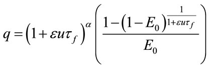
 (3)
(3)
where the inflow of HbR depends on the normalized oxygen extraction , since an increase in
  will increase [HbR] while reducing [HbO]. The outflow of HbR is proportional to the percentage of the HbR content
 . The core of the model is the physiccal necessity to largely increase CBF
  to achieve a small increase in oxygen delivery. An increase in cerebral blood flow is very closely linked to the underlying neuronal activity [34]. The model proposed by Buxton et al. [34] is very flexible with respect to the prediction of hemodynamic response parameters [5]. Here we have applied a similar model presented in Figure 1.
Balloon model is a nonlinear hemodynamic model. Due to the significant noise induced by measurements we have applied a stochastic hemodynamic system model to describe it. A continuous-discrete extended Kalman filter (Kalman filter for nonlinear systems) is used as a reasonable model to estimate the nonlinear states of the balloon model. The Balloon model [22] is an input-state-output model with two state variables volume (v) and deoxy-hemoglobin content (q). The input to the system is blood flow (fin) and the output is the BOLD signal (y). The BOLD signal is partitioned into an extra and intravascular component, weighted by their respecttive volumes. These signal components depend on the deoxyhemoglobin content and render the signal a nonlinear function of v and q. The effect of flow on v and q determines the output and it is these effects that are the essence of the Balloon model: Increases in flow effecttively inflate a venous “balloon” such that deoxygenated blood is diluted and expelled at a greater rate. The clearance of deoxyhemoglobin reduces intravoxel dephasing and engenders an increase in signal.
Before the balloon has inflated sufficiently the expulsion and dilution may be insufficient to counteract the increased delivery of deoxygenated blood to the venous compartment and an “early dip” in signal may be expressed. After the flow has peaked, and the balloon has relaxed again, reduced clearance and dilution contribute to the poststimulus undershoot commonly observed. This is a simple and plausible model that is predicated on a minimal set of assumptions and is relates closely to the windkessel formulation [35]. Furthermore the predictions of the Balloon model concur with the steady-state models of Hoge and colleagues, and their studies of the relationship between blood flow and oxygen consumption in human visual cortex [36].
The Balloon model is inherently nonlinear [2,16,37] and may account for the sorts of nonlinear interactions revealed by the Volterra formulation [37]. One simple test of this hypothesis is to see if the Volterra kernels associated with the Balloon model is comparable with those derived empirically. The Volterra kernels estimated in Friston et al. [2] clearly did not use flow as input
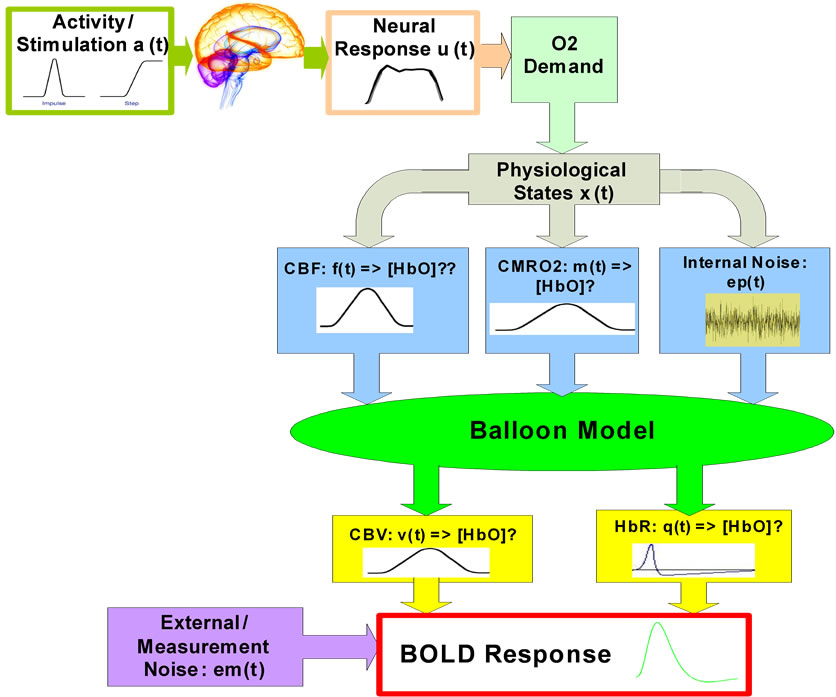
Figure 1. Overview diagram of the applied brain hemodynamic model.
because flow is not measurable with BOLD fMRI. The input comprises a stimulus function as an index of synaptic activity. In order to evaluate the Balloon model in terms of these Volterra kernels it has to be extended to accommodate the dynamics of how flow is coupled to a synaptic activity encoded in the stimulus function.
In summary the Balloon model deals with the link between flow and BOLD signal. By extending the model to cover the dynamic coupling of synaptic activity and flow a complete model, relating experimentally induced changes in neuronal activity to BOLD signal, obtains. The input-output behavior of this model can be compared to the real brain in terms of their respective Volterra kernels.
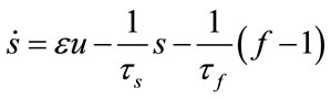
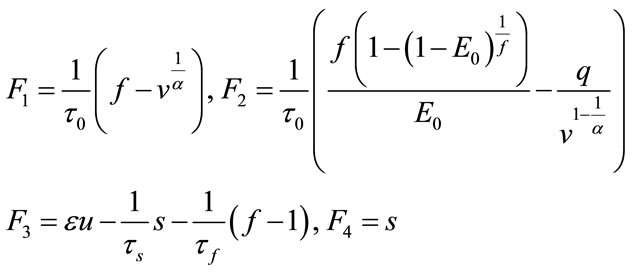
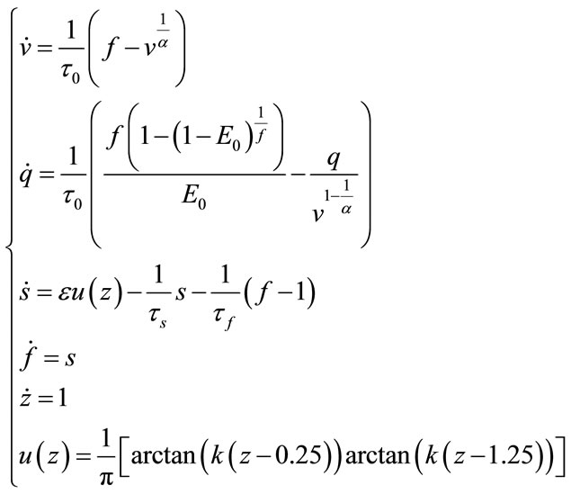
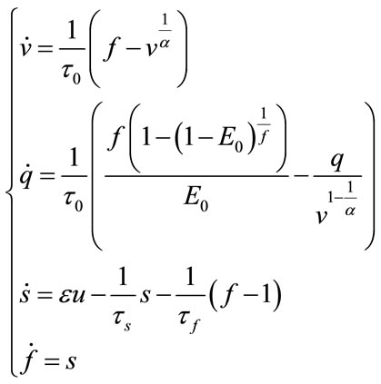
In 1998 Buxton published an input-output model which provided a relation between blood flow and BOLD signal and called it balloon model. Balloon model is a nonlinear dynamic state space model which is composed of two main states and one output which is the - BOLD signal. But one of its variables depends on another state and a neural activity signal (input). So, we have four states which are v cerebral blood volume (CBV), q deoxyhaemoglobin content, s flow inducing signal, f cerebral blood flow (CBF). These equations are acquired from the magnetic properties of hemoglobin which is diamagnetic for oxy-hemoglobin and paramagnetic for deoxy-hemoglobin. Using the electromagnetic equations around a cylinder and variation with oxygen saturation we can find the balloon model. The balloon model is a hemodynamic model. The neural activity signal u is the input of the model. The mathematical expression of hemodynamic balloon model is as follows:
 (4)
(4)
 (5)
(5)
 (6)
(6)
 (7)
(7)
And output which is BOLD signal is:
 (8)
(8)
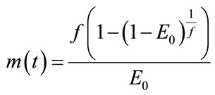
We can measure a new parameter , which is CMRO2 normalized to baseline too.
 (9)
(9)
In this model  is baseline oxygen extraction fraction,
  is baseline blood volume,
  is weight for deoxyHb change and
  is the weight for blood volume.
  is the mean transit time of the venous compartment, α is the stiffness component of the balloon model,
  is the signal decay time constant,
  is the autoregulatory time constant, and ɛ is the neuronal efficacy. Now, we can describe the state space equations as a nonlinear dynamic system. The state of the system is a vector:
 (10)
(10)
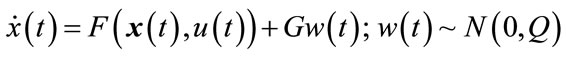
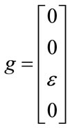
We can write the state space equation as a nonlinear form with an additional noise, which is a stochastic nonlinear dynamical system.
 (11)
(11)
 (12)
(12)
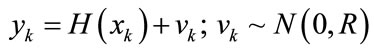
This model includes perturbation and measurement noise, because of weak signal of fMRI. In this state space equation,  is the state which is dependent on time (note that all of the states in the balloon model are time dependent but for simplicity we haven’t shown them in the balloon model),
  is input stimulus,
  is the perturbation noise (a white noise) which has mean 0 and variance Q. vk is measurement noise which is a white noise with mean 0 and variance R.
3.2. The Extended Kalman Filter
Extended Kalman filter is a nonlinear version of Kalman filter using for nonlinear dynamic systems. So, we estimate the states of balloon model using continuous-discrete extended Kalman filter. Suppose that a nonlinear stochastic dynamical system is described by:
 (13)
(13)
 (14)
(14)
and
 (15)
(15)
 ,
,  are independent Gaussian sequences having the following properties:
 ;
; ;
;
 ;
; 
 ;
; 
Prediction:
 (16)
(16)
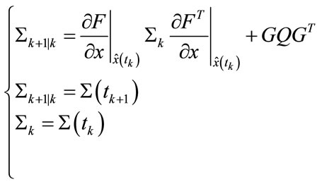 (17)
(17)
Update:
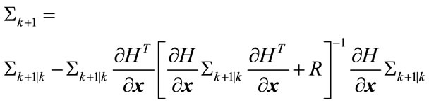 (18)
(18)
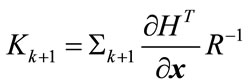 (19)
(19)
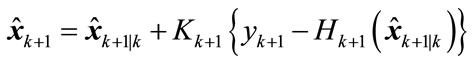 (20)
(20)
Initialization:
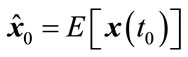 (21)
(21)
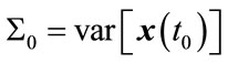 (22)
(22)
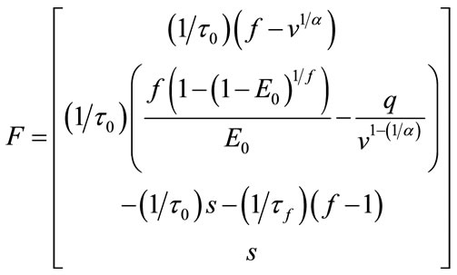
For the balloon model, we use the extended Kalman filter to predict BOLD signal. So, we should implement the Kalman filter equations according to the balloon model. First, the Jacobian matrix is needed which can be written as:
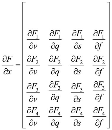 (23)
(23)
where:
 (24)
(24)
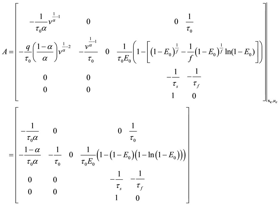
So, the Jacobian matrix will be written as:
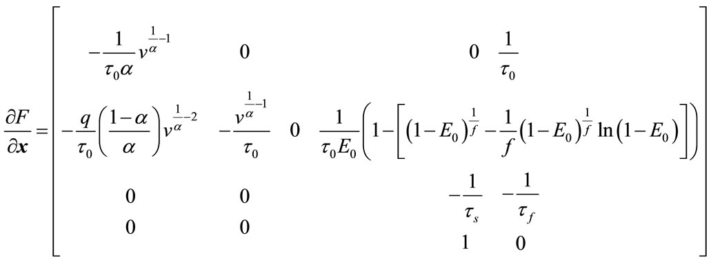 (25)
(25)
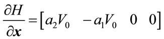
also, we need to calculate :
:
 (26)
(26)
 (27)
(27)
Other parts of the extended Kalman filter are very clear to calculate according to the above representations.
3.3. Neural Activity Dynamics
The input signal u in the balloon model is the neural activity and it is created by a square stimulus signal . The relation between the neural activity and the stimulus signal can be stated by:
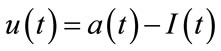 (28)
(28)
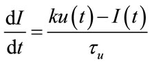 (29)
(29)
where  is the stimulus signal and
  is an inhibitory feedback signal and k is a gain factor.
  is a time constant. So, first the neural activity
  will be produced from
  and then use neural activity as an input to the balloon model. The
  is a step function as represented in Figure 2 by red line. In this figure the blue line signal is the neural activity and obtained by the
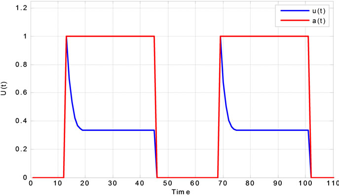
Figure 2. Neural activity response to a step function.
above differential equation. There are several models for neural activity. For example one simple estimation for neural activity is . In this model the neural activity is estimated to be same as stimulus.
3.4. Nonlinear Controller
In this part a nonlinear controller for the balloon model will be proposed. At the first the equilibrium point should be calculated. At the equilibrium point the derivative of state will be zero and we obtain these values for the equilibrium point:
 (30)
(30)
 (31)
(31)
 (32)
(32)
 (33)
(33)
As we see the important parameters for the equilibrium point are ,
, ![]() ,
,  ,
, ![]() and we have investigated their effects in the bifurcation analysis.
and we have investigated their effects in the bifurcation analysis.
4. SIMULATION AND EXPERIMENTAL RESULTS
4.1. Simulation Parameters
The values of parameters in the model are set to achieve the least error:
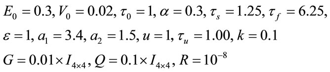
And the initial value is: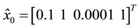 ,
, .
.
4.2. Simulated Results
By implementing the extended Kalman filter the BOLD signal will be estimated: First we simulated the balloon model in simulink (Figure 3(a)), and produced reasonable neural activity input and then we obtained output as a BOLD signal. Then we added white noise to this signal in order to produce a noisy BOLD signal. Using the extended Kalman filter in MATLAB to the noisy signal, produced a signal, which follows the measurements. The results are shown in the Figures 3(a) and (b).
4.3. Experimental Results
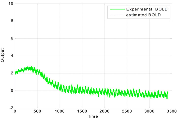
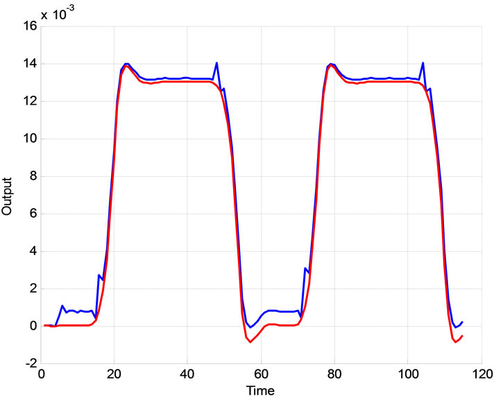
The proposed system is verified using real clinical measured data plotted in Figure 4. The extended Kalman filter is used to estimate the BOLD signal.
4.4. Bifurcation Analysis
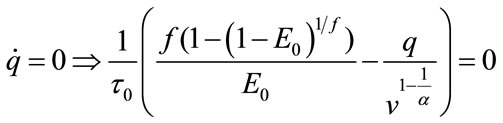
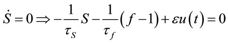
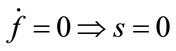
Bifurcation analysis investigates the stability of the system under change of parameters. Thus, it is important to first investigate nonlinear stability of the system and then use MatCont for Bifurcation analysis. For bifurcation analysis first the equilibrium point should be calculated. At the equilibrium point the derivative of state will be zero:
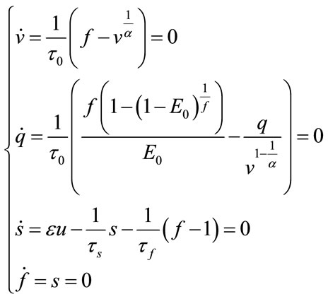 (34)
(34)
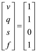
and we obtain these values for the equilibrium point:
 (35)
(35)
As we see the important parameters for the equilibrium point are ,
, ![]() ,
,  ,
, ![]() and we have investigated their effects in the bifurcation analysis. Now, we put this equilibrium point in the Jacobian matrix and then find the eigenvalues of that matrix to investigate the nonlinear stability of balloon model for different parameters.
and we have investigated their effects in the bifurcation analysis. Now, we put this equilibrium point in the Jacobian matrix and then find the eigenvalues of that matrix to investigate the nonlinear stability of balloon model for different parameters.
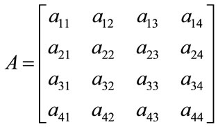
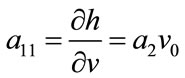
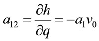
The Jacobian matrix is:
 (a)
(a) (b)
(b) (c)
(c)
Figure 3. (a) Simulink diagram presenting dynamics of the hemodynamic model; (b) The BOLD signal and its estimation; (c) The estimation error of BOLD signal.
 (a)
(a)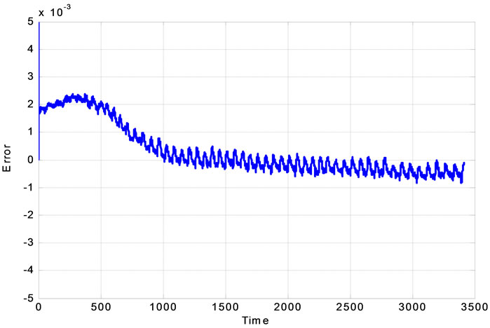 (b)
(b)
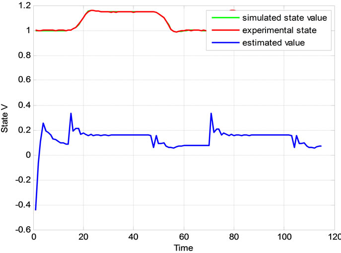
Figure 4. (a) Real experimental measurement of output data and its estimation; (b) the Experimental error.
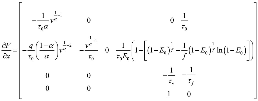
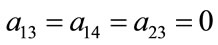
So, for the equilibrium point the Jacobian matrix is:

The eigen-values of this matrix will be:
 (36)
(36)
As we see all of the eigen-values are negative and this system for every choice of parameters is always stable. This is very interesting achievement regarding to the stability characteristics of the proposed system to describe the hemodynamic parameters. These eigenvalues depend on 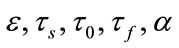 and independent of
 . For the bifurcation analysis, in this paper MatCont is used to analyse stability of the system with change of different effective parameters of the system. Using MatCont forces us to change and augment our system to ODE’s type. So, we have:
 (37)
(37)
So, by this definition, we start to get results for bifurcation analysis: These figures show the behaviour of real part of eigenvalues which are important for Bifurcation analysis versus the variation of parameters.
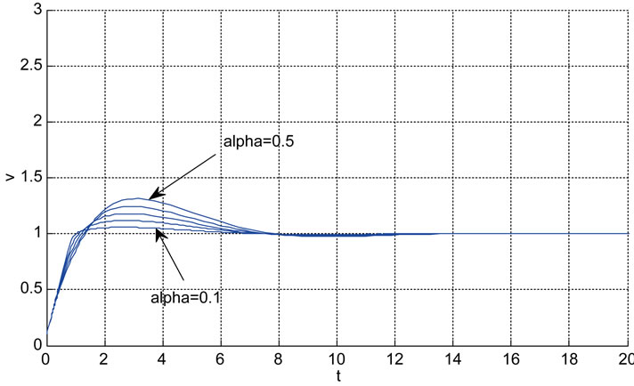
Relation between eigenvalues and different parameters are depicted in Figures 5-10 shows the effects of changing the model parameters on the evoked BOLD response. Figure 11 shows the simulated, measured, and the estimated BOLD signals. The Figure 12 shows the variation of states v cerebral blood volume and q deoxyhemoglobin versus the parameters of the model. As we see, the effect of τs is very important especially on the time of reaching to steady state. For higher τs the system will reach to steady state later and, so if our purpose is to reach to steady state condition, we should have a small τs.
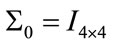
4.5. The Effect of Initialized Variance 
As it is supposed when the initialized variance ( ) increases that is the initial conditions are unknown and it causes that the contribution of measurements in the update equation increases which results the faster convergence. For higher
  especially when the system starts, Kalman gain is more than the case of the lower
  and this can be seen in Figure 13. The convergence is slower when
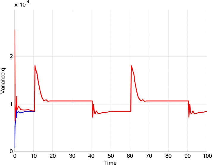
  is low which means we trust to the initial values. Figure 14 shows the typical variation of variance of state q for different values of
 . It is obvious that after convergence, the variance of estimated parameter is acceptable.
4.6. The Effect of R
Due to the relationship between R and Kalman gain, when the level of the noise at the measured value increases(R increases) the gain will decrease and the contribution of measurement in the update equation will decrease. Therefore slower convergence is a direct result
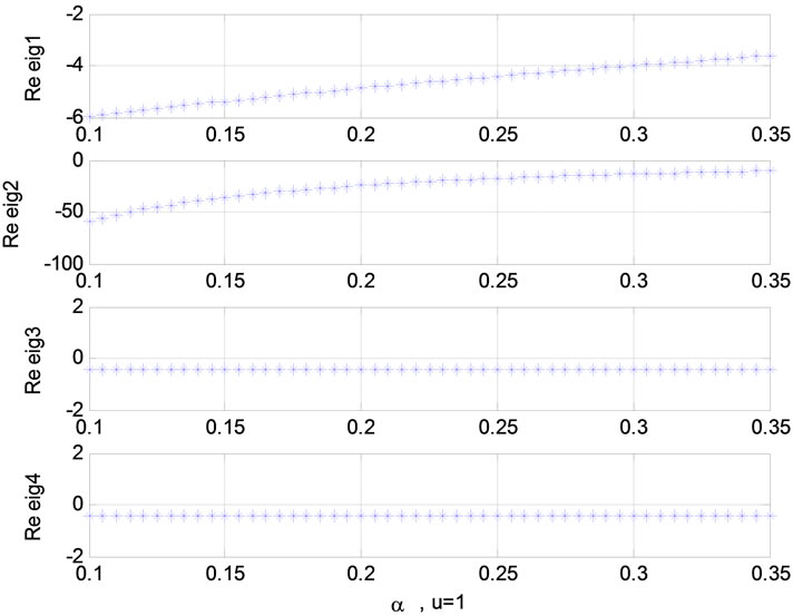

Figure 5. Relation between eigenvalues and stimulation function (u); Relation between eigenvalues and α in present of stimulation.
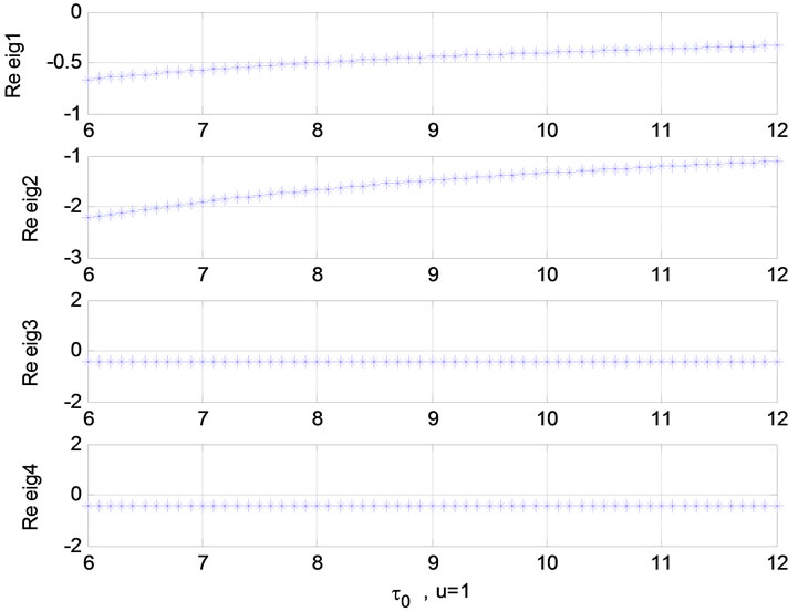
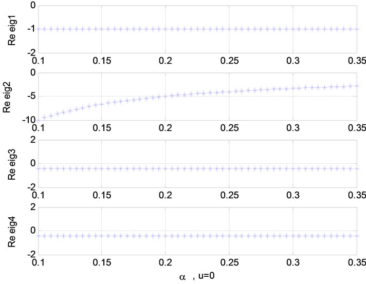
Figure 6. Relation between eigenvalues and α without stimulation; Relation between eigenvalues and τ0 (u = 1).
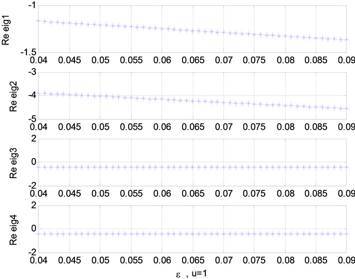
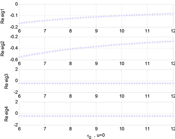
Figure 7. Relation between eigenvalues and ![]() (u = 0); Relation between eigenvalues and ε (u = 1).
(u = 0); Relation between eigenvalues and ε (u = 1).
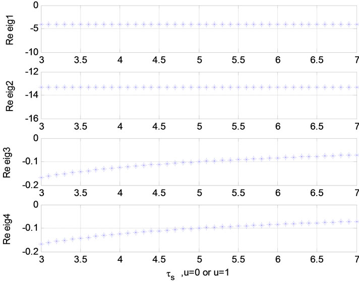
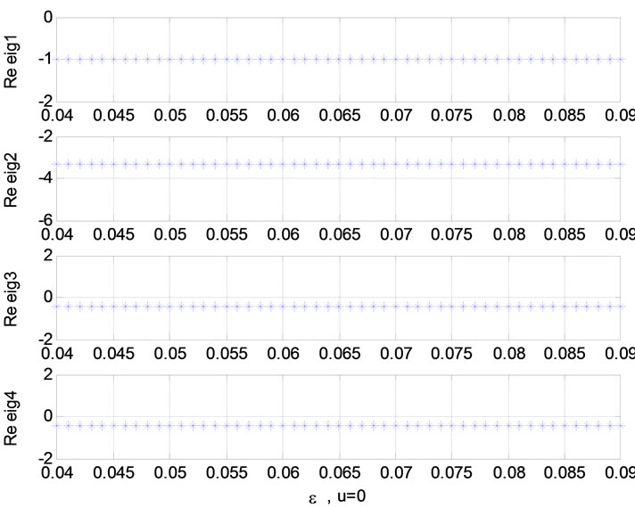
Figure 8. Relation between eigenvalues and ε (u = 0); Relation between eigenvalues and ![]() (u = 0 or 1).
(u = 0 or 1).

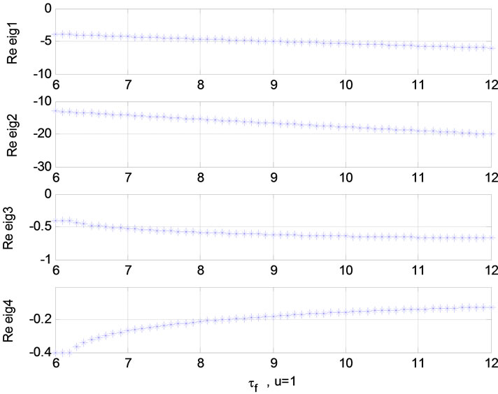
Figure 9. Relation between eigenvalues and  (u = 1); Relation between eigenvalues and
  (u = 0).
 (a)
(a) (b)
(b)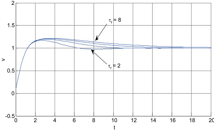 (c)
(c)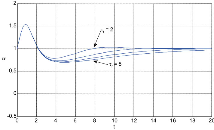 (d)
(d) (e)
(e)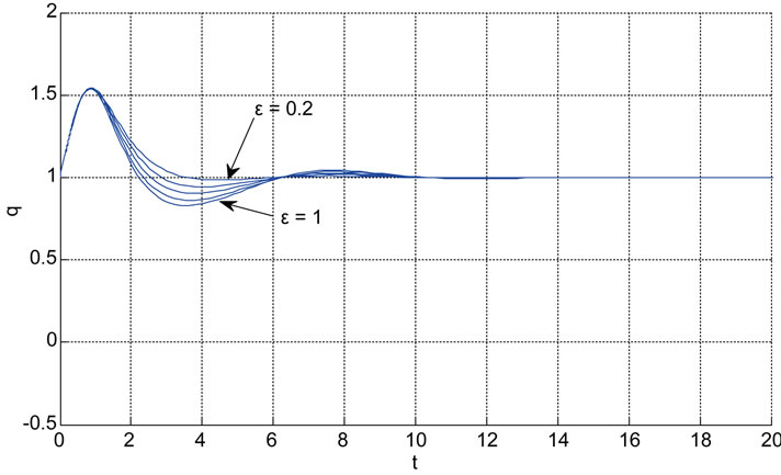 (f)
(f) (g)
(g) (h)
(h)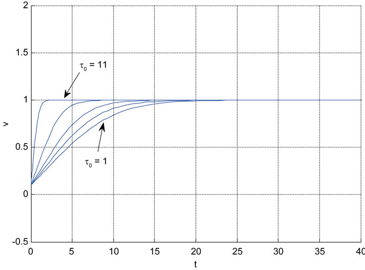 (i)
(i)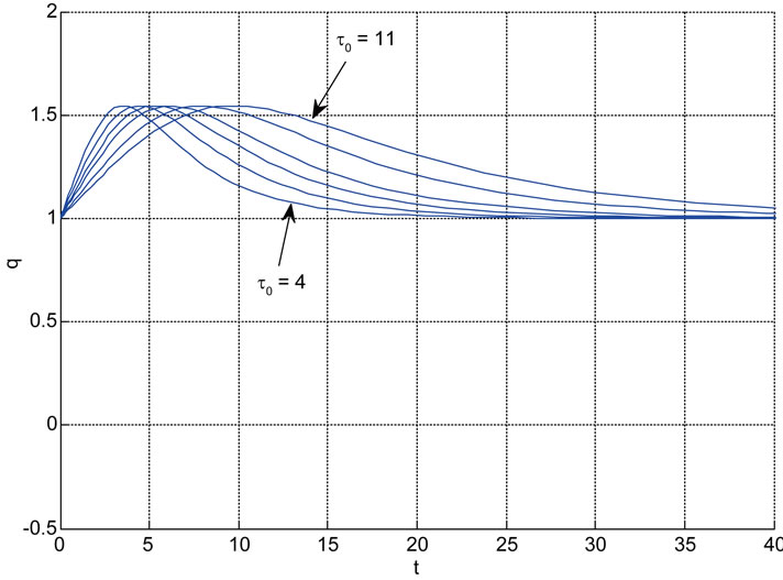 (j)
(j)
Figure 10. The effects of changing the model parameters on the evoked BOLD response. Solid lines correspond to the response after changing the parameter and the broken line is the response for the original parameter values (the e is the neuronal efficacy, τs is signal decay, τf is autoregulation, τ0 is transit time, α is stiffness, and E0 is oxygen extraction as in [2]).
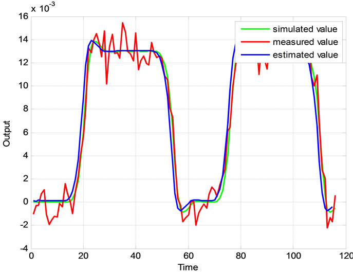
Figure 11. The simulated, measured, and the estimated BOLD signals.
of the higher noise level at the output.
4.7. Stability
The nonlinear stability of balloon model (directly) is investigated before and is proved that it is stable in Section 4.4. Bifurcation Analysis. Here in this part the stability is represented based on linearization of the balloon model.According to our review and investigations, we found that the stability, observability, and controllability that we were followed are based on non-linear model directly and our investigations are true. This is a simpler model of stability when all of the eigenvalues of the system are negative . In this situation, the system is linearizable and it is possible to linearize the state space equation and then use the definition of stability, observability, and controllability in the linear case.
 (a)
(a) (b)
(b)
Figure 12. Comparison between simulated and experimental results. (a)The blood volume v and (b) The deoxyhaemoglobin content q.
 (a)
(a)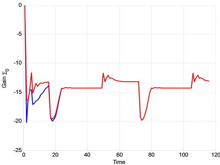 (b)
(b)
Figure 13. The effect of Σ0 on the extended Kalman filter Blue: Σ0 = I, R = 0.00012, Red: Σ0 = 0.001.I, R = 0.00012; The effect of Σ0 on the extended Kalman filter Blue: Σ0 = 0.00001I, R = 0.00012, Red: Σ0 = 0.001I, R = 0.00012.
As we know, the balloon model is described as:
 (38)
(38)
And output which is BOLD signal is:
The linear model is in the form of:

where:
 ;
; ;
; ;
; 
and  are the equilibrium point.
 ;
; ;
; 
The eigenvalues of A are:
 ;
; ;
; 
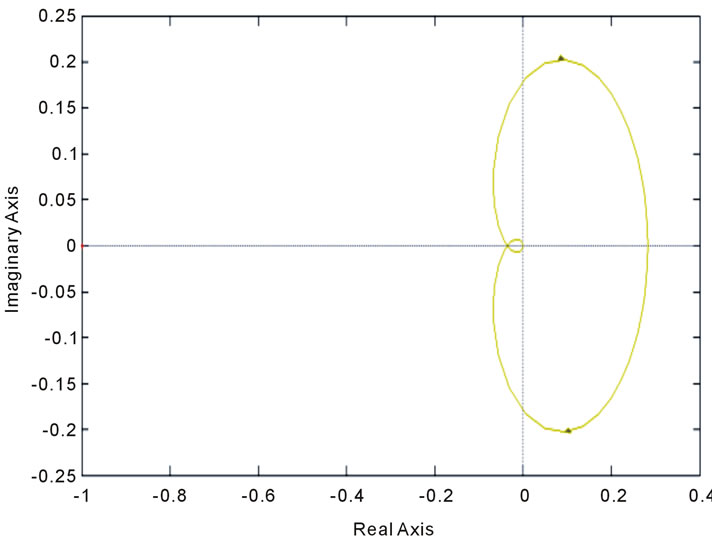
All of these eigenvalues are negative and equal to the case of nonlinear stability analysis when u = 0. So, the system is stable. Root-Locus and Nyquist curves are plotted in Figure 15.
4.8. Controllability and Observability
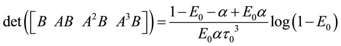
The linear and nonlinear controllability and observability has been investigated at this section. Here first the model is linearized and then controllability and observability have been verified. Based on the controllability matrix  and observability index
 , we can determine their determinant to investigate if the system is controllable and observable or not. The determinant of each matrix is as followed:
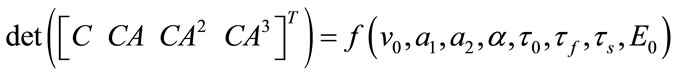
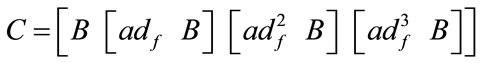
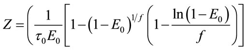
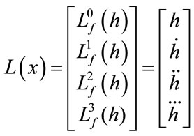
And for nonlinear observability the controlability and observability of the system using balloon model without linearizing the dynamic system (nonlinear controllability and observability) have been investigated as follow. For nonlinear controllability we have:
 ;
; ;
;
 ;
; 
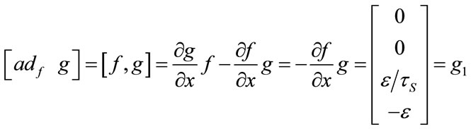 ;
;

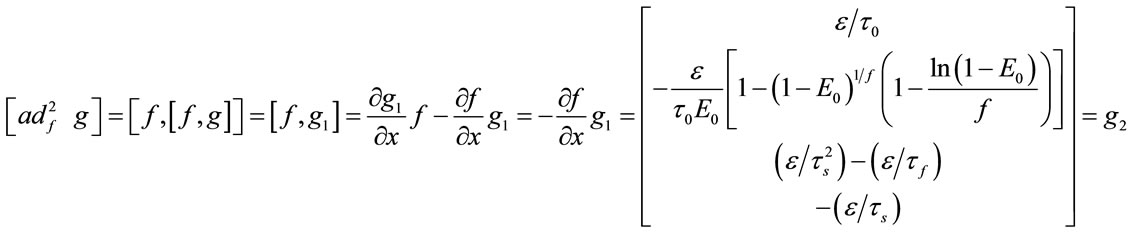
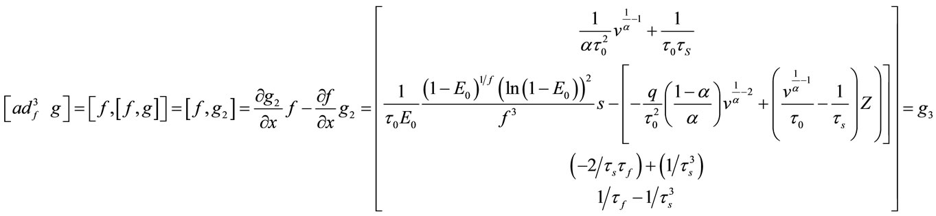
where:

 (a)(b)
Figure 14. The effect of R on the extended Kalman filter Blue: Σ0 = I, R = 0.0012, Red: Σ0 = I, R = 0.000012; The effect of Q on the output of the extended Kalman filter Blue: Σ0 = I, R = 0.000012, Q = 0.1.I, Red: Σ0 = I, R = 0.000012, Q = 0.001.I.
 (a)
(a)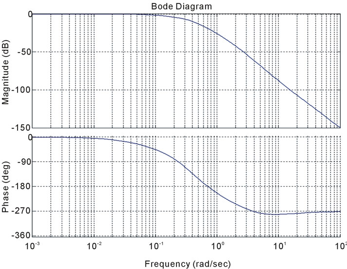 (b)
(b) (c)
(c) (d)
(d)
Figure 15. Stability analysis using (a): Bode diagram, (b): nyquist, (c): open-loop root locus, and (d): closed-loop root locus.
The determination of the hemodynamic observables (BOLD, CBF, [HbR], oxyhemoglobin concentration [HbO] and total hemoglobin concentration [HbT]) is subject of this study. This technique with a better quantification and specificity has so far not been implemented in combined studies, giving hope to increase the homogeneity of observations in future experiments. The Equilibrium point is calculated as:
 ;
;
 ;
;
 ;
; 
 ;
; ;
;
The observability matrix is:
 ;
; 
where:
 ;
; ;
; ;
; ;
; ;
; ;
; ;
; ;
; ;
; ;
; ;
; ;
; ;
; ;
; ;
; ;
; 
As the observability and controllability of linear and nonlinear systems depend on many parameters, we have calculated them in equilibrium point and for the parameters before introduced in 4.1. It shows that for these values the system is controllable and observable.
5. CONCLUSION AND FUTURE WORK
We presented a state space model realization of the integrated version of the balloon model. In addition to the nonlinear filter techniques used in previous approaches [15-27,29] this new modeling can utilize the advantages of using more sophisticated and robust techniques in linear and nonlinear estimation. Proposed stochastic hemodynamic systems describe the brain neural activity according to balloon model. The continuous-discrete extended Kalman filter is used to estimate the nonlinear model states. The stability, controllability and observability of the proposed model are described based on the simulation and measurement data analysis. Up to our knowledge this is the first work on evaluation of these control parameters and introducing their practical impacts on clinical application. Surprisingly we realized that the system is always stable independent from any variation in blood flow and HbR/HbO variation. The observability and controllability characteristics are introduced as significant factors to be considered as an evaluation tool to verify the preference of different hemodynamic factors. The preferred factors then can be considered based on their specified priority for further diagnosis and monitoring in clinical applications. This model can also be efficiently applied in any monitoring and control platform include brain and for study of hemodynamic and brain imaging modalities such as pulse oximetry and functional near infra-red spectroscopy. The work is on progress to extend the proposed model to cover more hemodynamic and neural brain signals for real-time invivo applications.
6. ACKNOWLEDGEMENTS
We gratefully acknowledge the financial support from the Canadian Institutes of Health Research (CIHR) and the Heart and Stroke Foundation of Canada then the Canada Research Chair in smart medical devices and CMC Microsystems.
REFERENCES
- Johnston, L.A., Duff, E., Mareels, I. and Egan, G.F. (2008) Nonlinear estimation of the BOLD signal. NeuroImage, 40, 504-514. doi:10.1016/j.neuroimage.2007.11.024
- Friston, K.J., Mechelli, A., Turner, R. and Price, C.J. (2000) Nonlinear responses in fMRI: The balloon model, Volterra kernels, and other hemodynamics. NeuroImage, 12, 466-477. doi:10.1006/nimg.2000.0630
- Banaji, M., Mallet, A., Elwell, C.E., Nicholls, P. and Cooper, C.E. (2008) A model of brain circulation and metabolism: NIRS signal changes during physiological challenges. PLoS Computational Biology, 4, e1000212. doi:10.1371/journal.pcbi.1000212
- Aquino, K.M., Schira, M.M., Robinson, P.A., Drysdale, P.M. and Breakspear, M. (2012) Hemodynamic traveling waves in human visual cortex. PLoS Computational Biology, 8, e1002435. doi:10.1371/journal.pcbi.1002435
- Steinbrink, J., Villringer, A., Kempf, F., Haux, D., Boden, S. and Obrig, H. (2006) Illuminating the BOLD signal: Combined fMRI-fNIRS studies. Magnetic Resonance Imaging, 24, 495-505. doi:10.1016/j.mri.2005.12.034
- Schira, M.M., Tyler, C.W., Breakspear, M. and Spehar, B. (2009) The foveal confluence in human visual cortex. The Journal of Neuroscience, 29, 9050-9058. doi:10.1523/JNEUROSCI.1760-09
- Kamitani, Y. and Tong, F. (2005) Decoding the visual and subjective contents of the human brain. Nature Neuroscience, 8, 679-685. doi:10.1038/nn1444
- Strangman, G., Culver, J.P., Thompson, J.H. and Boas, D.A. (2002) A quantitative comparison of simultaneous BOLD fMRI and NIRS recordings during functional brain activation. NeuroImage, 17, 719-731. doi:10.1006/nimg.2002.1227
- Zheng, Y., Martindale, J., Johnston, D., Jones, M., Berwick, J. and Mayhew, J., (2002) A model of the hemodynamic response and oxygen delivery to brain. NeuroImage, 16, 617-637. doi:10.1006/nimg.2002.1078
- Logothetis, N.K., Pauls, J., Augath, M., Trinath, T., Oeltermann, A. (2001) Neurophysiological investigation of the basis of the fMRI signal. Nature, 412, 150-157. doi:10.1038/35084005
- Duncan, A., Meek, J.H., Clemence, M., Elwell, C.E., Tyszczuk, L., Cope, M., et al. (1995) Optical pathlength measurements on adult head, calf and forearm and the head of the newborn infant using phase resolved optical spectroscopy. Physics in Medicine and Biology, 40, 295- 304. doi:10.1088/0031-9155/40/2/007
- Kohl, M., Nolte, C., Heekeren, H.R., Horst, S., Scholz, U., Obrig, H., et al. (1998) Determination of the wavelength dependence of the differential pathlength factor from nearinfrared pulse signals, Physics in Medicine and Biology, 43, 1771-1782. doi:10.1088/0031-9155/43/6/028
- Daunizeau, J., Kiebel, S.J. and Friston, K.J. (2009) DyNnamic causal modelling of distributed electromagnetic responses. NeuroImage, 47, 590-601. doi:10.1016/j.neuroimage.2009.04.062
- Breakspear, M., Jirsa, V. and Deco, G. (2010) Computational models of the brain: From structure to function. NeuroImage, 52, 727-730. doi:10.1016/j.neuroimage.2010.05.061
- Buxton, R.B., Wong, E.C. and Frank, L.R. (1998) Dynamics of blood flow and oxygenation changes during brain activation: The balloon model. Magnetic Resonance in Medicine, 39, 855-864. doi:10.1002/mrm.1910390602
- Hettiarachchi, I.T., Pathirana, P.N. and Brotchie, P. (2010) A state space based approach in non-linear hemodynamic response modeling with fMRI data. IEEE Annual International Conference on Engineering in Medicine and Biology (EMBC), Buenos Aires, 31 August 2010-4 September 2010, 2391-2394. doi:10.1109/IEMBS.2010.5627400
- Glover, G.H. (1999) Deconvolution of Impulse Response in Event Related BOLD fMRI. NeuroImage, 9, 416-429.
- Dale, M.A. and Buckner, R.L. (1997) Selective averaging of rapidly presented individual trials using fMRI. Human Brain Mapping, 5, 329-390. doi:10.1002/(SICI)1097-0193
- Obata, T., Liu, T.T., Miller, K.L., Luh, W.-M., Wong, E.C., Frank, L.R. and Buxton, R.B. (2004) Discrepancies between BOLD and flow dynamics in primary and supplementary motor areas: Application of the balloon model to the interpretation of BOLD transients. NeuroImage, 21, 144-153. doi:10.1016/j.neuroimage.2003.08.040
- Fritson, K.J., Josephs, O., Rees, G. and Turner, R. (1998) Nonlinear event-related responses in fMRI. Magnetic Resonance in Medicine, 39, 41-52. doi:10.1002/mrm.1910390109
- Fritson, K.J., Jezzard P. and Turner, R. (1994) Analysis of functional MRI time series. Human Brain Mapping, 1, 153-171.
- Kong, Y.Z., et al. (2004) A model of the dynamic relationship between blood flow and volume changes during brain activation. Journal of Cerebral Blood Flow & Metabolism, 24, 1382-1392. doi:10.1097/01.WCB.0000141500.74439.53
- Deneux, T. and Faugeras, O. (2006) Using nonlinear models in fMRI data analysis: Model selection and activation detection. NeuroImage, 32, 1669-1689. doi:10.1016/j.neuroimage.2006.03.006
- Buxton, R.B., Uludağ, K., Dubowitz, D.J. and Liu, T.T. (2004) Modeling the hemodynamic response to brain activation. NeuroImage, 23, 220-233. doi:10.1016/j.neuroimage.2004.07.013
- Johnston, L.A., Duff, E., Mareels, I. and Egan, G.F. (2008) Nonlinear estimation of the BOLD signal. NeuroImage, 40, 504-514. doi:10.1016/j.neuroimage.2007.11.024
- Hu, Z., Zhao, X., Liu, H. and Shi, P. (2009) Nonlinear analysis of the BOLD signal. EURASIP Journal on Advances in Signal Processing, 2009, 1-14. doi:10.1155/2009/215409
- Engel, S.A., Glover, G.H. and Wandell, G.H. (1997) Retinotopic organization in human visual cortex and the spatial precision of functional MRI. Cerebral Cortex, 7, 181- 192. doi:10.1093/cercor/7.2.181
- Kriegeskorte, N., Cusack, R. and Bandettini, P. (2010) How does an fMRI voxel sample the neuronal activity pattern: Compact-kernel or complex spatiotemporal filter? NeuroImage, 49, 1965-1976. doi:10.1016/j.neuroimage.2009.09.059
- Magri, C., Schridde, U., Murayama, Y., Panzeri, S. and Logothetis, N.K. (2012) The amplitude and timing of the BOLD signal reflects the relationship between local field potential power at different frequencies. The Journal of Neuroscience, 32, 1395-1407. doi:10.1523/JNEUROSCI.3985-11.2012
- Bailey, C. J., Sanganahalli, B. G., Herman, P., Blumenfeld, H., Gjedde, A. and Hyder, F. (2012) Analysis of time and space invariance of BOLD responses in the rat visual system. Cerebral Cortex, In Press.
- doi:10.1093/cercor/bhs008
- Friston, K. J., Fletcher, P., Josephs, O., Holmes, A., Rugg, M.D. and Turner, R. (1998) Event-related fMRI: Characterizing differential responses. NeuroImage, 7, 30-40.
- doi:10.1006/nimg.1997.0306
- Javed, F., et al. (2012) Recent advances in the monitoring and control of haemodynamic variables during haemodialysis: A review. Physiological Measurement, 33, R1-R31. doi:10.1088/0967-3334/33/1/R1
- Javed, F., Savkin, A.V., Chan, G.S.H., Mackie, J.D. and Lovell, N.H. (2011) Identification and control for automated regulation of hemodynamic variables during hemodialysis. IEEE Transactions on Biomedical Engineering, 58, 1686-1697. doi:10.1109/TBME.2011.2110650
- Buxton, R.B., Uludağ, K., Dubowitz, D.J. and Liu, T.T. (2004) Modeling the hemodynamic response to brain activation. NeuroImage, 23, S220-S233. doi:10.1016/j.neuroimage.2004.07.013
- Mandeville, J.B., Marota, J.J., Ayata, C., Zararchuk, G., Moskowitz, M.A., Rosen, B. and Weisskoff, R.M. (1999) Evidence of a cerebrovascular postarteriole windkessel with delayed compliance. Journal of Cerebral Blood Flow & Metabolism, 19, 679-689. doi:10.1097/00004647-199906000-00012
- Hoge, R.D., Atkinson, J., Gill, B., Crelier, G.R., Marrett, S. and Pike, G.B. (1999) Linear coupling between cerebral blood flow and oxygen consumption in activated human cortex. Proceedings of the National Academy Sciences, 96, 9403-9408. doi:10.1073/pnas.96.16.9403
- Jacobsen, D.J. (2006) Hemodynamic modelling of BOLD fMRI: A machine learning approach. Ph.D. Thesis, Technical University of Denmark, Copenhagen. doi:10.1.1.85.3860