Intelligent Information Management
Vol.4 No.3(2012), Article ID:19352,7 pages DOI:10.4236/iim.2012.43007
The Asymptotic Study of Smooth Entropy Support Vector Regression
School of Electronics and Information, Shanghai Technical Institute of Electronics and Information, Shanghai, P. R. China
Email: jamhu8@sohu.com
Received December 4, 2011; revised February 28, 2012; accepted February 28, 2012
Keywords: Support Vector Machine; SSVR; Entropy Function; Asymptotic Solution; Forecasting
ABSTRACT
In this paper, a novel formulation, smooth entropy support vector regression (SESVR), is proposed, which is a smooth unconstrained optimization reformulation of the traditional linear programming associated with an ε-insensitive support vector regression. An entropy penalty function is substituted for the plus function to make the objective function continuous ,and a new algorithm involving the Newton-Armijo algorithm proposed to solve the SESVR converge globally to the solution. Theoretically, we give a brief convergence proof to our algorithm. The advantages of our presented algorithm are that we only need to solve a system of linear equations iteratively instead of solving a convex quadratic program, as is the case with a conventional SVR, and lessen the influence of the penalty parameter C in our model. In order to show the efficiency of our algorithm, we employ it to forecast an actual electricity power short-term load. The experimental results show that the presented algorithm, SESVR, plays better precisely and effectively than SVMlight and LIBSVR in stochastic time series forecasting.
1. Introduction
Support vector machines (SVMs), based on statistical learning theory, are powerful tools for pattern classifications and regression problems [1,2] and have been employed in engineering practices [3,4]. The basic SVM model, maximal margin classifier, needs to solve a constrained optimization mathematical programming, i.e., seek for the hyperplane  to realizes the maximal margin hyperplane with geometric margin [2]:
 (1)
(1)
subject to ,
, .
.
For a given linearly separable training sample  . Generally, a simple and direct method to solve the above SVM model is to transform this optimization problem into its corresponding dual model with some constraint relations as a Lagrangian problem. Traditionally, the researchers usually transfer a constraint optimization problem into unconstrained problems to deal with SVM problems. However, after transformation, the corresponding unconstrained problem with an important plus function
  is not differentiable, so we can not use the traditional fast Newton method to directly solve. Fortunately, smoothing methods have been extensively used for solving important mathematical programming problems [5-8]. So, it is natural that we used the smoothing method to deal with SVM problems. The nature of the smoothing method is to construct a continue polynomial to substitute the plus function
  [9-15].
Chen and Mangasarian applied the penalty function to solve the SVM [16]. It is well known that the exact penalty function is better than inexact penalty function for the constrained optimization problems [18]. Meanwhile, Smooth support vector regression (SSVR) is seldom researched except Lee and Wang [17]. So, in this paper, we propose a new smooth entropy support vector regression (SESVR) model using an exact penalty function which is different from the approximating function in [16], and study its asymptotic solution approaching the solution of primal problem.
The proposed SESVR model has strong mathematical properties, such as strong convexity and infinitely often differentiability. To demonstrate the proposed SESVR’s capability in solving regression problems, we employ SESVR to forecast on power short-term load forecasting from the actual electric network. We also compared our SESVR model with SVMlight [19] and LIBSVM [20] in the aspect of forecast accuracies.
This paper is organized as follows. Standard SVM and SSVM are briefly reviewed in Section 2. In Section 3, a novel SESVR model is proposed. In Section 4, we analyze the asymptotic solution of SESVR. We use the synthetic data and actual electric power load to test the proposed SESVR and give a brief analysis in Section 5. Finally, some conclusions are drawn in Section 6.
2. A Brief Review of SSVM
2.1. Standard SVM
Given a training sample set  with size of l, xi is a column vector,
 . The learning objective is to construct a hyperplane to correctly classify the test samples.
  represents the classification hyperplane with two different data classes, the sign of data is determined by the following equations:
 ,
, ;
; ,
, 
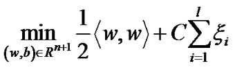
SVM is mainly used to construct a classification hyperplane to separate two different kind samples and maximize the separation margin. For the nonlinear problem, it is necessary to introduce penalty parameter C and nonnegative slack variable , The larger C is, the more severe penalty is. Therefore, the quadratic optimization problem can be obtained as following:
 (2)
(2)
subject to
 ,
, .
.
 ,
, .
.
2.2. Smooth Support Vector Machine (SSVM)
Given a database consisting of m points in the  -dimensional real space
 , which are represented by a
  matrix, where the
  row of the matrix A corresponds to the
  data point. Two class data
  and
and  belong to positive (+1) and negative (−1), respectively. A
  diagonal matrix D with ones or negative ones along its diagonal can be used to specify the membership of each point. In other words,
  depending on whether the label of
  data point is +1 or –1.
Combining the two constraint conditions of problem (2), we obtain
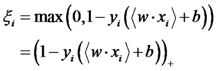 (3)
(3)
where  is a plus function defined as follows
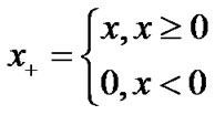 .
.
We substitute Equation (3) into Equation (2), and convert Equation (2) into an equivalent SVM (4) which is an unconstrained optimization problem.
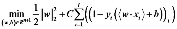 (4)
(4)
The above function (4) has a unique solution. Function  is not differentiable and unsmooth, therefore, it cannot be solved using conventional Newton optimization method, because it always requires the objective function’s gradient and Hessian matrix exist. Lee and Mangasarian modified the second part of function (4) and made it smooth to build a smooth unconstrained problem similar to unsmooth unconstrained problem. To do that, Lee introduced an approximation of an unsmooth function
 , which is the integral function of Sigmoid function[9,16]:
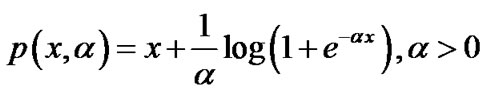 (5)
(5)
Obviously,  approach the plus function
  as
as  tends to infinity, therefore, the unconstrained optimization problem (4) is equivalent to the following smooth support vector machine (SSVM) optimization problem (6):
 (6)
(6)
The simple lemma that bounds the square difference between the plus function  and its smooth approximation
 .
.
Lemma 2.1 [9] For  and
and ,
,
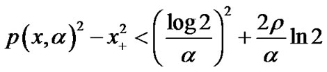 , where
  is p function of (5) with smoothing parameter
 .
.
As the smoothing parameter α approaches infinity, the unique solution of our smooth problem (6) using NewtonArmijo Algorithm approaches the unique solution of the equivalent SVM problem (2).
Theorem 2.2 [9] Let  be a sequence generated by Newton-Armijo Algorithm and
  be the unique solution of problem (6).
1) The sequence  converges to the unique solution (
 ) from any initial point (w0, b0) in
 .
.
2) For any initial point , there exists an integer
  such that the stepsize
  of Newton-Armijo Algorithm equals 1 for
  and the sequence
  converges to
 .
.
Recently, some smooth functions are constructed to replace the plus function , for example, tangent circular arc smooth piecewise function in [11], cubic spline interpolation function and Hermite interpolation polynomial in [12], two piecewise smooth functions (1PSSVM, 2PSSVM) in [13] and so on.
3. The Proposed SESVR Model
Given a data set S which consists of l points in n-dimensional real space  and l observations of real value associated with each point, that is,
We would like to find a linear or nonlinear regression function,  , tolerating a small error in fitting this given data set. This can be achieved by utilizing the
  - insensitive loss function that sets an
  -insensitive “tube” around the data, within which errors are discarded. Also, applying the idea of support vector machines (SVMs) [2]. The function
  is made as flat as possible in fitting the training data set. The idea of representing the solution by means of a small subset of training points has enormous computational advantages. The
  -insensitive loss function maintains that advantages, while still ensuring the existence of a global minimum and the optimization of a reliable generalization bound.
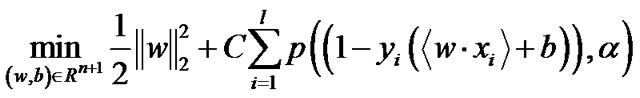
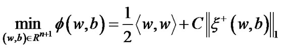
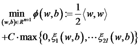
This linear regression problem can be formulated as an unconstrained minimization problem given as follows:
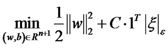 (7)
(7)
where, 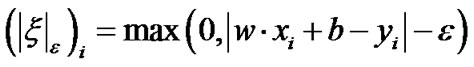 ,
, .
.
That represents the fitting errors and the positive control parameter C here weights the tradeoff between the fitting errors and the flatness of the linear regression function . To deal with the
  -insensitive loss function in the objective function of the above minimization problem, conventionally, it is reformulated as a constrained minimization problem defined as follows:

Subject to
 (8)
(8)
This formulation (8), which is equivalent to the formulation (7), is a convex quadratic minimization problem with  free variables, 2 l nonnegative variables, and 2 l inequality constraints. However, more variables and constraints in the formulation enlarges the problem size and could increase computational complexity for solving the regression problem.
We denote

and . Adopting Fletcher’s nonlinearly undifferentiable precise penalty method [21], we obtain the equivalent unconstraint optimization problem:
 (9)
(9)
Lemma 3.1 [22]  is an arbitrary point in
 ,
,  is a Lagrange multiplier vector. If parameter C satisfies
  and
and . Then the 2nd order optimal sufficient condition is equivalent between the optimization problem (9) and problem (8) in the point
 . where
  is a dual norm of
 .
.
In term of Lemma 3.1, inter-dual norm  and
and when the trade-off penalty factor C satisfying
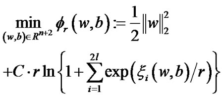
 , we can solve the following optimal problem:
 (10)
(10)
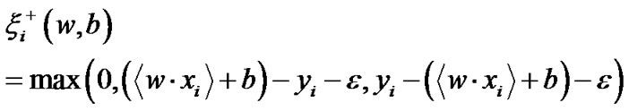
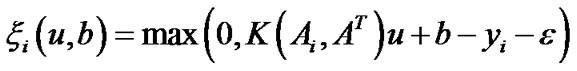
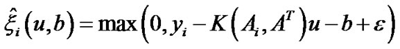
and obtain a feasible solution of the optimization problem (9). However, maximum function 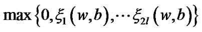 is not smooth and undifferentiable, so that, we can not directly utilize Newton gradient descent method. We employ the following smooth entropy function
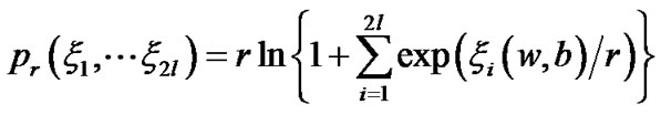 and substitute it for approximating maximum function
  .
.
Lemma 3.2 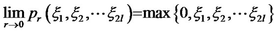
for arbitrary .
.
Then, we obtain the smooth and differentiable optimization model (11) which is equivalent to problem (9):
 (11)
(11)
We call the above problem (11) a smooth entropy support vector regression (SESVR).
4. The Asymptotic Analysis of SESVR
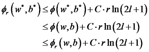
The proposed SESVR problem (11) is an infinitely differentiable optimization issue, and can be solved using Newton iterating algorithm. We hope solve the problem (11) instead of the problem (9), however, so far, we don’t know the solution relations between the problem (11) and the primal SVR problem (8). In fact, when although the solution of the primal problem (8) is not the optimal solution of the problem (11), we can prove that the convergence bound between the solution of the problem (11) and the solution of the problem (9) is controlled by smoothing parameter r i.e..
Theorem 4.1 Suppose that  is a optimal solution of problem (9), and
  is Lagrange multiplier vector, if
 , then for an arbitrary point
  and a given small
 , we have
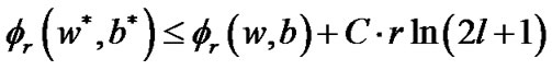 (12)
(12)
Proof. Because point  is the optimal solution of problem (9), and
  is Lagrange multiplier vector, we obtain the Karush-Kuhn-Tucher complementarity conditions:
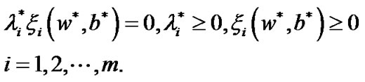 (13)
(13)
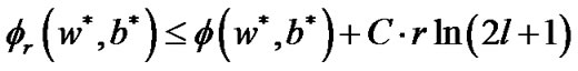
From Lemma 3.1, we know  is the optimal solution of problem (10), so, we obtain inequality (14)
On the other hand, for any given point , penalty parameter
 , and arbitrary small constant
 , we have
 (15)
(15)
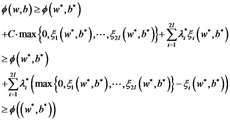
Considering  being a feasible solution, then we get
 (16)
(16)
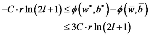
From Equations (14), (15), and (16), we know
Then, the theorem 4.1 is correct.
Theorem 4.2 Suppose that  is a optimal solution of problem (9),
  is Lagrange multiplier vectorand
  is the optimal solution of problem (11), if
 , then
 (17)
(17)
The proof is similar to theorem 3.4 in [22], so we abandon the redundant proof.
Theorem 4.2 shows that the solution of SESVR (11) approaches the solution of primal problem (8) as the smoothing parameter . By making use of this results and taking advantage of the twice differentiability of the objective function, we prescribe a globally convergent algorithm 4.3 based on Newton-Armijo algorithm for solving (11) as follows.
Algorithm 4.3 Start with any choice of initial point , and stop if
  satisfy
 and
and  for a given sufficiently small constant
 .
.
Step 1: Initialize ,
, .
.
Step 2: For , using Newton-Armijo algorithm [9,16], we solve the unconstraint optimization problem:
Step 3: Let . If
. If  is a feasible solution of (11), then
 , otherwise,
 .
.
From Algorithm 4.3, we can easily validate the following facts.
1)  and
and
 as
as .
.
2)  and for an arbitrary
 ,
,
 .
.
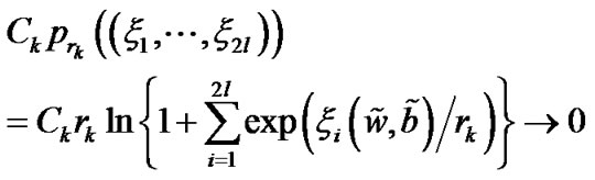
3) If the sequences  contain a non-feasible infinite sub-sequence, then
 .
.
With finitely iterating, the sequence  of Algorithm 4.3 globally converge to the unique solution based on the following Lemma 4.4 - 4.5 and Theorem 4.6.
Lemma 4.4 The sequence  is boundary and all the corresponding cluster points are feasible points of problem (9).
Lemma 4.5 Any cluster point of sequence  is the optimal solution of problem (9).
Theorem 4.6 Let {(wk, bk)} be a sequence generated by Algorithm 4.3 and ( ) be the unique solution of problem (9).
1. The sequences  converge to unique solution
  from any initial point
 .
.
2. For any initial point , there exists an integer
  such that the stepsize
  of Newton-Armijo Algorithm equals 1 for
  and the sequence {(wk, bk)} converges to
 .
.
Lemma 4.5, Lemma 4.6 and Theorem 4.6 can be inferred from [9,18]. In the above discussion, we construct the smooth entropy support vector regression model for a linear regression function in fitting the given training data points under the criterion that minimizes the squares of the  -insensitive loss function. That is approximating
  by a linear function of the form:
 (18)
(18)
where  and
and  are parameters to be determined by minimizing the objective function in (11). Applying the duality theorem in convex minimization problem [23],
  can be represented by
  for some
 . Hence, we have
 (19)
(19)
This motivated the nonlinear support vector regression model. In order to generalize our results from the linear case to nonlinear case, we employ the kernel technique that has been used extensively in kernel-based learning algorithms [1,2].
We simply replace the  in (19) by a nonlinear kernel matrix K(A, AT), where
and  is a nonlinear kernel function. Using the same loss criterion with the linear case, this will give us the nonlinear support vector regression formulation as follows:
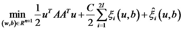 (20)
(20)
where
 ,
,
 ,
,
 .
.
 is a kernel map from
  to
to . We solve the optimal solution (20) using Algorithm 4.3, and obtain parameters
  and
and . Then the regression function is
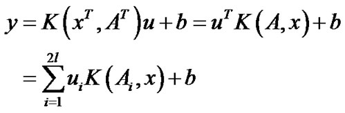 (21)
(21)
5. Experimental Results and Analysis
In order to test the efficiency of our proposed smooth entropy support vector regressions, we utilize SESVR to forecast electricity power short term load and compared the results with the conventional SVMlight [19] and LIBSVM [20].
All experiments were run on a personal computer, which consisted of a 1.9 GHz AMD dual core processor and 960 megabytes of memory. Based on the first order optimality conditions of unconstrained convex minimization problem, our stop criterion for the proposed model was satisfied when the gradient of the objective function is less than  and select
 . We implemented SESVR in C++ programming. In the experiments, 2- norm relative error was chosen to evaluate the tolerance between the predicted values and the actual values. For an actual value
  and the predicted vector
 , the 1- norm relative error of two vectors
  and
and  was defined as follows:
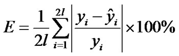 (22)
(22)
Aim to evaluate how well each method generalized to unseen data, we split the entire data set into two parts, the training set and testing set. The training data was used to generate the regression function that is learning from training data; the testing set, which is not involved in the training procedure, was used to evaluate the prediction ability of the resulting regression function. A smaller testing error indicates a better prediction ability. We performed tenfold cross-validation on each data set and reported the average testing error in our numerical results.
Our actual power load data and its corresponding weather data come from HuaiNan electric network from April 2004 to August 2004, sampling frequency is one times each hour, sampling days is 120, so we gain 2880 (120 × 24) training data. We use trained SESVR model to forecast the load of August 10 2005. It is know that summer season influence power load more drastically than other three seasons, it is why we sample load from summer season, meanwhile, we can study whether or not weather influence and how to influence electricity load. The numerical results of short-term load forecasting were also included in following Table 1.
From Table 1 and Figure 1, we can find out our proposed SESVR model is a feasible forecasting method for electric power short-term load, If we generated the training samples for SESVR including the weather temperatures, the relative error is 1.28%, otherwise the error is 3.06%. so, the weather temperatures can upgrade forecasting accuracies, moreover, we can see that the relative errors of night time is bigger than that of daytime. On the other hand, we find out the penalty parameter C in Algorithm 4.3 increases monotonously, so Algorithm 4.3 is stable, however, SVMlight and LIBSVM are influenced by penalty parameter C. In order to gain the optimal solutions of SVMlight and LIBSVM, we must tune C carefully. This increases the computational complexity. With regard to this point, Algorithm 4.3 is superior to SVMlight and LIBSVM.
Figure 2 illustrates the tenfold numerical results and comparisons of our proposed SESVR, SVM, LIBSVM. The experimental results demonstrated that our proposed SESVR model is a powerful tool for forecast electric power short-term load, and better precise and effective

Figure 1. The electricity load forecasting results using our proposed SESVR model. Blue line, Red line, and Green line show the actual load, forecasting load with no temperature, and forecasting load with temperature, respectively.
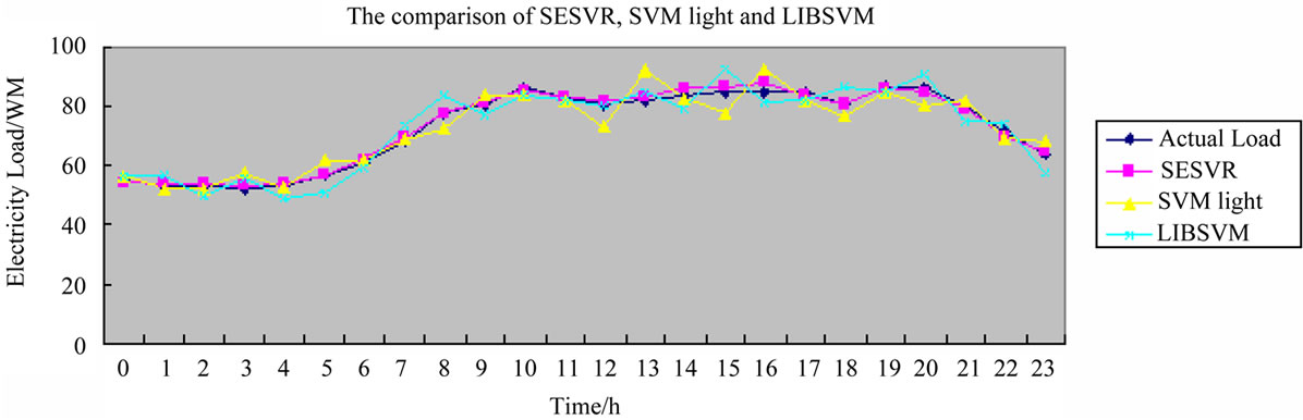
Figure 2. The electricity load forecasting comparison of SESVR, SVMlight, LIBSVM. Blue line shows the actual load, read line represents the forecasting load using our proposed regression model SESVR, Yellow line and Green line illustrate the forecasting loads using SVMlight and LIBSVM model, respectively.


Table 1. The load forecasting result on 10 August 2005.
than LIBSVM and SVMlight model.
6. Conclusions
We have proposed a novel formulation, SESVR, which is a smooth unconstrained optimization reformulation of the traditional linear programming associated with an ε-I nsensitive support vector regression. We have employed an entropy penalty function to substitute it for the plus function to avoid objective discontinuous. We have proposed a new algorithm involving a very fast Newton-Armijo algorithm to solve the SESVR that has been shown convergent globally to the solution. In our algorithm, the penalty parameter C is creasing monotonously, the influence to SESVR performance is smaller than foregoing SVMlight and LIBSVM. Theoretically, we have given a brief convergence proof to our algorithm.
In order to show the efficiency of our algorithm, we employ it to forecast an actual electricity power shortterm load. The experimental results show that the proposed SESVR is effective and precise, and plays better performances than SVMlight and LIBSVR in stochastic time series forecasting. Moreover, an advantage of our proposed SESVR algorithm is that we only need to solve a system of linear equations iteratively instead of solving a convex quadratic program, as is the case with a conventional SVR.
REFERENCES
- C. V. Gustavo, G. Juan and G. P. Gabriel, “On the Suitable Domain for SVM Training in Image Coding,” Journal of Machine Learning Research, Vol. 9, No. 1, 2008, pp. 49-66.
- F. Chang, C. Y. Guo and X. R. Lin, “Tree Decomposition for Large-Scale SVM Problems,” Journal of Machine Learning Research, Vol. 11, No. 10, 2010, pp. 2935-2972.
- Y. H. Kong, W. Cai Wei and W. He, “Power Quality Disturbance Signal Classification Using Support Vector Machine Based on Feature Combination,” Journal of North China Electric Power University, Vol. 37, No. 4, 2010, pp. 72-77.
- J. Zhe, “Research on Power Load Forecasting Base on Support Vector Machines,” Computer Simulation, 2010, No. 8, pp. 282-285.
- B. Chen and P. T. Harker, “Smooth Approximations to Nonlinear Complementarity Problems,” SIAM Journal of Optimization, Vol. 7, No. 2, 1997, pp. 403-420. doi:10.1137/S1052623495280615
- C. H. Chen and O. L. Mangasarian, “Smoothing Methods for Convex Inequalities and Linear Complementarity Problems,” Mathematical Programming, Vol. 71, No. 1, 1995, pp. 51-69. doi:10.1007/BF01592244
- C. H. Chen and O. L. Mangasarian, “A Class of Smoothing Functions for Nonlinear and Mixed Complementarity Problems,” Computational Optimization and Applications, Vol. 5, No. 2, 1996, pp. 97-138. doi:10.1007/BF00249052
- X. Chen, L. Qi and D. Sun, “Global and Superlinear Convergence of the Smoothing Newton Method and Its Application to General Box Constrained Variational Inequalities,” Mathematics of Computation, Vol. 67, No. 222, 1998, pp. 519-540. doi:10.1090/S0025-5718-98-00932-6
- Y. J. Lee and O. L. Mangasarin, “SSVM: A Smooth Support Vector Machine for Classification,” Computational Optimization and Applications, Vol. 20, No. 1, 2010, pp. 5-22. doi:10.1023/A:1011215321374
- Z. Q. Meng, G. G. Zhou and Y. H. Zhu, “A Smoothing Support Vector Machine Based on Exact Penalty Function,” Lecture Notes in Artificial Intelligence, 2005, Vol. 3801, pp.568-573.
- Y. F. Fan, D. X. Zhang and H. C. He, “Tangent Circular Arc Smooth SVM(TCA-SSVM) Research,” 2008 Congress on Image and Signal Processing, Sanya, 27-30 May 2008, pp. 646-648. doi:10.1109/CISP.2008.112
- Y. F. Fan, D. X. Zhang and H. C. He, “Smooth SVM Research: A Polynomial-Based Approach,” The 9th International Conference on Information and Communications Security, Singapore, 10-13 December 2007, pp. 983-988.
- L. K. Lao, C. D. Lin, H. Peng, et al., “A Study on Piecewise Polynomial Smooth Approximation to the Plus Function,” The 9th International Conference on Control, Automation, Robotics and Vision, Singapore, 5-8 December 2066, pp. 342-347.
- J. Z. Xiong, T. M. Hu and G. G. Li, “A Comparative Study of Three Smooth SVM Classifiers,” Proceedings of the 6th World Congress on Intelligent Control and Automation, Dalian, 21-23 June 2006, pp. 5962-5966.
- P. A. Forero, A. C. Georgios and B. Giannakis, “ConsensusBased Distributed Support Vector Machines,” Journal of Machine Learning Research, Vol. 11, No. 5, 2010, pp. 1663- 1707.
- C. H. Chen and O. L. Mangasarian, “Smoothing Methods for Convex Inequalities and Linear Complementarity Problems,” Mathematical Programming, Vol. 71, No. 1, 1995, pp. 51-69. doi:10.1007/BF01592244
- Y. J. Lee, W. F. Hsieh and C. M. Huang, “ε-SSVR: A Smooth Support Vector Machine for ε-Insensitive Regression,” Knowledge and Data Engineering, Vol. 17, No. 5, 2005, pp. 678-695. doi:10.1109/TKDE.2005.77
- S. H. Peng and X. S. Li, “The asymptotic analysis of quasi-exact penalty function method,” Journal of Computational Mathematics, 2007, Vol. 29, No. 1, pp. 47-56.
- T. Joachims, “SVMlight,” 2010. http://svmlight. joachims .org
- C.-C. Chang and C.-J. Lin, “LIBSVM: A Library for Support Vector Machines,” 2010. http://www.csie.ntu. edu.tw/~cjlin/libsvm
- R. Fletcher, “Practical methods of optimization,” John Wiley & Sons, New York, 1981.
- O. L. Mangasarian and D. R. Musicant, “Successive overrelaxation for support vector machines,” IEEE Transactions on Neural Networks, Vol. 10, No. 5, 2010, pp. 1032- 1037. doi:10.1109/72.788643 ftp://ftp.cs.wisc.edu/math-prog/tech-reports/98-18.ps
- Y. W. Chang, C. J. Hsieh and K. W. Chang, “Training and Testing Low-degree Polynomial Data Mappings via Linear SVM,” Journal of Machine Learning Research, Vol. 11, No. 4, 2010, pp. 1471-1490.