Intelligent Information Management
Vol.4 No.2(2012), Article ID:18213,9 pages DOI:10.4236/iim.2012.42004
Bayesian and Non-Bayesian Estimation of the Inverse Weibull Model Based on Generalized Order Statistics
Department of Mathematics, Sohag University, Sohag, Egypt
Email: ahmhamed@hotmail.com, ahmed.abdelah@science.sohag.edu.eg
Received September 21, 2011; revised December 10, 2011; accepted December 20, 2011
Keywords: Inverse Weibull Distribution; Generalized Order Statistics; Record Values; Progressive Type-II Censored; Balanced Type Loss Function; Bootstrap Estimation
ABSTRACT
The concept of generalized order statistics has been introduced as a unified approach to a variety of models of ordered random variables with different interpretations. In this paper, we develop methodology for constructing inference based on n selected generalized order statistics (GOS) from inverse Weibull distribution (IWD), Bayesian and non-Bayesian approaches have been used to obtain the estimators of the parameters and reliability function. We have examined Bayes estimates under various losses such as the balanced squared error (balanced SEL) and balanced LINEX loss functions are considered. We show that Bayes estimate under balanced SEL and balanced LINEX loss functions are more general, which include the symmetric and asymmetric losses as special cases. This was done under assumption of discrete-continuous mixture prior for the unknown model parameters. The parametric bootstrap method has been used to construct confidence interval for the parameters and reliability function. Progressively type-II censored and k-record values as a special case of GOS are considered. Finally a practical example using real data set was used for illustration.
1. Introduction
Udo Kamps [1,2] has introduced GOS as random variables having certain joint density function, which includes as a special case the joint density functions of many models of ordered random variables such as ordinary order statistics (OS) (David [3], Castillo [4] and Arnold, Balakrishnan and Nagaraja [5]), sequential order statistics (SOS) (Cramer and Kamps [6,7]), record values, Kth record values, and Pfeifer’s records (Nevzorov [8] and Ahsanullah [9]), Progressive Type-II censoring order statistics (PCOS) (Soliman [10-13], Balakrishnan and Asgharzadeh [14], and Sarhan, Ammar and Abuammoh [15]). The structural similarities of these models are based on the similarity of their joint density function. Therefore, all of these models are contained in the model of GOS.
For Bayesian estimates, the performance depends on the form of the prior distribution and the loss function assumed. The prior information can be expressed by the experimenter, who has some belifs about the parameters of his parametric model. Traditionally, most authors use the simple quadratic loss function and obtain the posterior mean as the Bayesian estimate. However, in practice, the real loss function is often not symmetric. For example, the conesquences of overestimates, in loss of human life, are much more serious than the consequences of underestimates. In this case an asymmetric loss function is more appropriate. Recently, many authors consider asymmetric loss functions in reliability, such as [Wahed [16], Alicja [17], Abd Ellah [18-20] and Sultan [21].
In this paper based on n selected GOS from the inverse Weibull model, we consider the problem of Bayesian and non-Bayesian estimation for parameters and reliability function of the model. This was done under assumption of discrete-continous mixture prior for the unknown parameters. It well know that in Bayesian setting, for making optimum decision, importance should be given on the choice of loss function and not just the choice of prior distribution. So, the results are presented under the balanced versions of symmetric and asymmetric loss functions. Progressively type-II censored and record values as a special case of GOS are considered. The rest of paper is organized as follows. In Section 2, we first present some preliminaries.
2. Preliminaries
2.1. The Model and the Concept of the GOS
The IWD plays an important role in many applications, including the dynamic components of diesel engines and several data set such as the times to breakdown of an insulating fluid subject to the action of a constant tension; see Nelson [22]. Calabria and Pulcini [23] provide an interpretation of the IWD in the context of the load-strength relationship for a component. Recently, Maswadah [24] has fitted the IWD to the flood data reported in Dumonceaux and Antle [25]. For more details on the IWD, see, for example Murthy et al. [26]. The two parameter IWD has probability density function (pdf) cumulative distribution function (cdf) and reliability function S(t) which are given respectively as
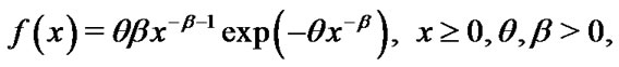 (1)
(1)
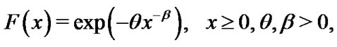 (2)
(2)
and the reliability function at time t is
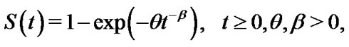 (3)
(3)
where  and
and  are scale and shape parameters respectively.
We recall the concept of GOS (cf. Kamps [1]).
Let  and
and  then the random variables

are called the generalized order statistics if their joint pdf is given by
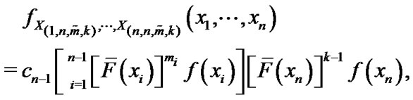 (4)
(4)
For , where
2.2. Balanced Type Loss Functions
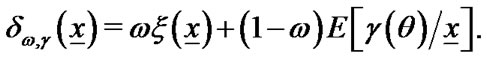
The class of balanced type loss function (BLF) we can write it in the form (see Ahmadi et al. [27]).
 (5)
(5)
where  estimating of parameter
 ,
,  a prior target estimator of
 ,
, ,
, being as arbitrary loss function in estimating
  by
by  and
and  suitable positive weight function. In this paper we shall use balanced squared error loss (balanced SEL) and balanced LINEX loss function to illustrate Bayesian estimation of parameters of inverse Weibull.
2.2.1. Balanced Squared Error Loss Function
The balanced SLE is obtained with the choice of
 and
and  in (5), and given by
 (6)
(6)
and the Bayes estimation of  under
under  is given by
 (7)
(7)
2.2.2. Balanced LINEX Loss Function
The balanced LINEX loss function with shape parameter , is obtained with the choice of
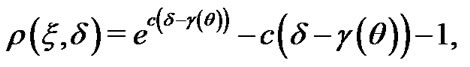 and
and  in (5), and given by
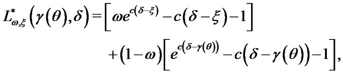 (8)
(8)
and the Bayes estimation of  under
under  is given by
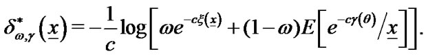 (9)
(9)
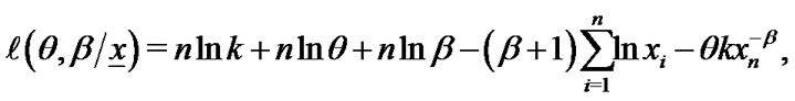
3. Maximum Likelihood Estimation (MLE)
Let 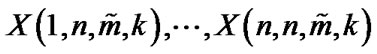 are n GOS drawn from inverse Weibull distribution whose pdf is given by (1), based on this set of GOS the log-likelihood function is
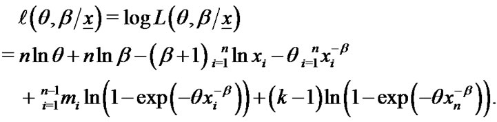 (10)
(10)
If both of the parameters  and
and  are unknowntheir MLEs,
  and
and  can be obtained by solving the following likelihood equations
 (11)
(11)
 (12)
(12)
The required estimates  and
and  are to be found by solving simultaneously the two Equations (11) and (12). Clearly that the calculation of the MLE requires iterative procedures. We can use the well known Newton-Raphson technique. By moving any point along in the direction determined by the information matrix and the first derivative of the log-likelihood function, we can iteratively improved the starting estimates to MLE, for details see Lawless [28]. For a given t, the corresponding MLE
  of the reliability function
  my be obtained by replacing
  and
and  by
by  and
and  in (4).
3.1. Special Cases
In general, it is not easy to find a natural interpretation of generalized order statistics in terms of observed random samples. So, an interesting special cases such as the progressive Type II censored order statistics and record values have been used. These models are the most applicable general models of ordered random variables and is useful in reliability and life time studies. Several authors have addressed inferential issues based on progressive Type-II censored samples (for example, see Balakrishnan and Sandhu [14], Aggarwala and Balakrishnan [29] Ng et al. [30], Balakrishnan et al. [31] and Soliman [10-13]. One may refer to Balakrishnan [32,33] for a recent overview of various developments relating to progressive censoring. Also, record values arise in a wide variety of practical situations. Examples include industrial stress testing, meteorological analysis, hydrology, seismology, sporting and athletic events, and oil and mining surveys. Properties of record values have been studied extensively in the literature. Interested readers may refer to the books by Nevzorov [8] and Arnold et al. [34,35].
In this section we will consider two special cases of GOS, namely, the progressively Type-II censored sample and lower record values.
3.1.1. Progressively Type-II Censored Data
A progressively Type-II censored sample is observed as follows: n units are placed on a life-testing experiment and only m ≤ n are completely observed until failure. The censoring occurs progressively in m stages. The m stages are failure times of m completely observed units. At the time of the first failure (the first stage), R1 of (n – 1) surviving units are randomly withdrawn from the experiment, R2 of the (n – R1 – 2) surviving units are withdrawn at the time of the second failure (the second stage) and so on. Finally, at the time of the mth failure (the mth stage), all the remaining (Rm – n – m – R1 – – Rm–1) surviving units are withdrawn. We will refer this to as progressively Type-II censoring scheme (R1, R2,
  , Rm) Then, we shall denote the m completely observed failure times by
The progressively Type-II censored sample 
 with censoring scheme
  and
and
 is a special case of the GOS with the parameters
 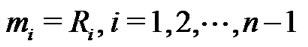 and
and 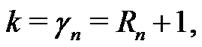 see Burkschat et al. [36].
From Equations (11) and (12) the required estimates
 and
and  in progressively Type-II censored are to be found by solving simultaneously the following two equations
 (13)
(13)
 (14)
(14)
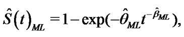
The ML estimate of reliability  is given by
 (15)
(15)
where  and
and  are be found from the numerical solution of the Equations (13) and (14).
3.1.2. Lower k-Record Values
Let  be a sequence of independent and identically (iid) continuous random variables with cumulative distribution function (cdf)
  and probability density function (pdf)
  An observation
  is defined to be an lower record if
  for every
  and an analogous definition can be given for upper records ( with the inequality being reversed ). The record values is special case of GOS, in which if we put
 and replacing
  by
by  in (10), then the log-likehood of lower k-record values is given by
 (16)
(16)
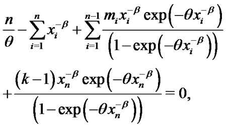
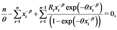
the ML estimates of  and
and  can be obtained from (16) by solving the following two equations as then
 (17)
(17)
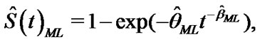
The ML estimate of reliability  is given by
 (18)
(18)
where  and
and  are given by (17).
4. Bayes Estimation
In this section, we estimate the two parameters  and
and  of IWD and The reliability
  based on GOS by considering both of balanced SEL and balanced LINEX loss function. Progressively type-II censored and k-record values as a special case of GOS are considered.
4.1. Bayes Estimation Based on GOS
When both of the two parameters  and
and  are assumed to be unknown, Soland [37] considered a family of joint prior distributions that places continuous distributions on the scale parameter and discrete distributions on the shape parameter.
Suppose that the shape parameter  is restricted to a finite number of values
  with respective prior probabilities
  such that
and  Further, suppose that conditional upon
 ,
,  has a natural gamma
 prior, with a density
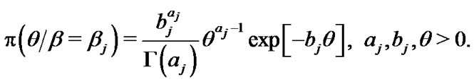 (19)
(19)
by using the Bayes theorem, the conditional posterior density function of  is given by
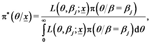 (20)
(20)
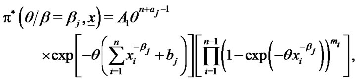
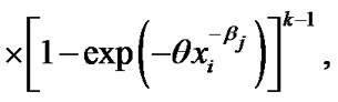 (21)
(21)
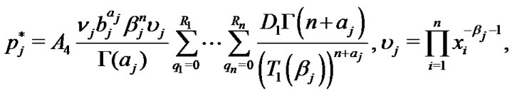
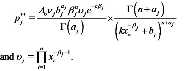
where 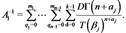 (22)
(22)
On applying the discrete version of Bayes theorem, the marginal probability distribution of  is given by
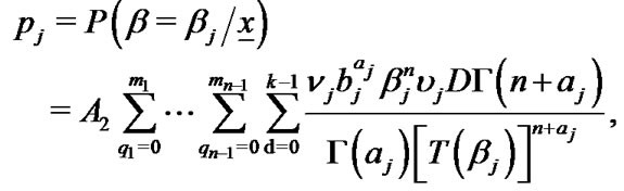 (23)
(23)
where
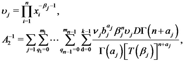 (24)
(24)
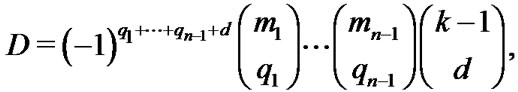
and 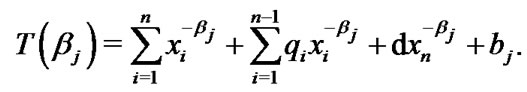 (25)
(25)
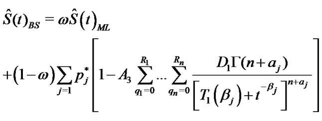
4.1.1. Bayes Estimation Based on Balanced SEL
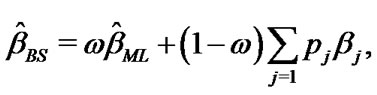
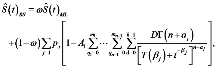
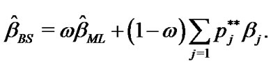
From (21) the Bayes estimates of ,
,  and
and  in GOS under balanced SEL can be obtained, respectively as
 (26)
(26)
 (27)
(27)
and
 (28)
(28)
where  and
and  are to be found by solving (11) and (12),
  A1, pj and
  are given respectively, by (15), (22), (23) and (25).
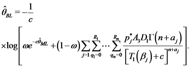
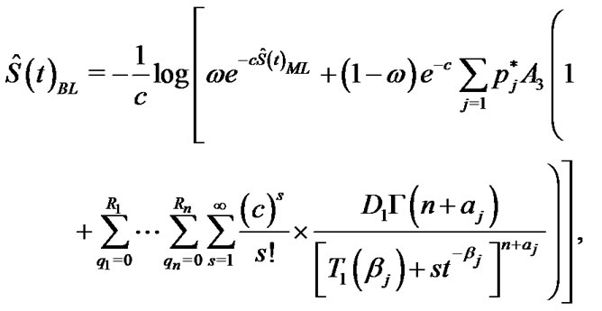
4.1.2. Bayes Estimation Based on Balanced LINEX Loss Function
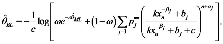
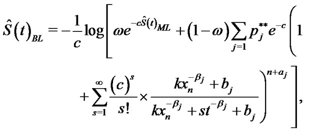
From (21) the Bayes estimates of ,
,  and
and  in GOS under balanced LINEX loss function can be obtained, respectively as
 (29)
(29)
 (30)
(30)
and
 (31)
(31)
where  and
and  are to be found by solving (11) and (12),
  A1, pj and
  are given respectively, by (15), (22) , (23) and (25).
4.2. Special Cases
In this subsection we will consider two special cases of gos, the progressively type-II censored sample and lower record values.
4.2.1. Progressively Type-II Censored Data
From Equations (26), (27) and (28) the Bayes estimates of ,
,  and
and  in progressively type-II censored data under balanced SEL, are given respectively by
 (32)
(32)
 (33)
(33)
and
 (34)
(34)
And From Equations (29), (30) and (31) the Bayes estimates of ,
,  and
and  in progressively type-II censored data under balanced LINEX loss function, given respectively by
 (35)
(35)
 (36)
(36)
and
 (37)
(37)
where
and 
 (38)
(38)
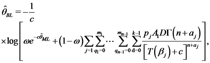
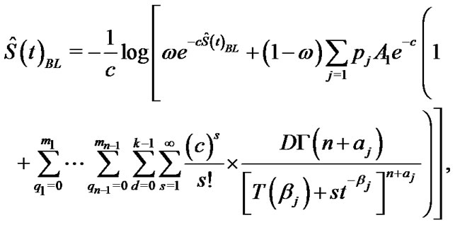
4.2.2. Lower k-Record Values
From (21), (22) and (27) in Lower k-record values the Bayes estimates of ,
,  and
and  under balanced SEL, given respectively by
 (39)
(39)
 (40)
(40)
and
 (41)
(41)
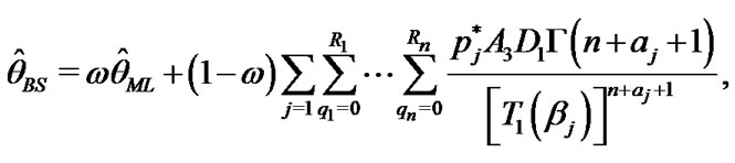
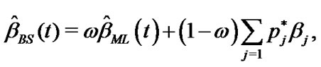
Similarly From (21), (22) and (27) in Lower k-record values the Bayes estimates of 
 and
and  under balanced LINEX loss function respectively, are given
 (42)
(42)
 (43)
(43)
and
 (44)
(44)
where
 (45)
(45)
5. Bootstrap Statistical Inference
The bootstrap is a resembling method for statistical inference. It is commonly used to estimate confidence intervals, but it can also be used to estimate bias and variance of an estimator or calibrate hypothesis tests. Bootstrapping is carried out by having an original data set  and sampling from an estimate of the cumulative distribution function (cfd) of
  such that there are H re-sampled data sets. The re-sampled data set will be denoted as Xi = (Xi1, Xi2,
  , Xin), i = 1, 2,
  , H. Inferences for the quantity
 , where
 is the vector of parameters, generally employ a test statistic, denoted as
 . In order to estimate the sampling distribution of
 , two methods are employed, the nonparametric and parametric bootstrap methods. The parametric bootstrap method involves having a mathematical model whose parameters that completely determine the probability density function (pdf) of
 , while the nonparametric one is used when there is not an explicitly given mathematical model to use, but it is assumed that the re-sampled data sets are independently and identically distributed (iid). The following algorithm to describe the percentile bootstrap method as:
Algorithm A: Percentile bootstrap algorithm 1) From an original data set , draw H independent bootstrap samples
 ,
,  ,
,  ,
,  with replacement, each of size n.
2) Compute  and
and  , i = 1, 2,
 , H in progrisseve type II censored from numerical solution of (13) and (14), and from numerical solution of (17) in lower record values.
3) Calculate the mean of all values in  and
and .
.
4) Sort the values  and
and  in ascending order to obtain the bootstrap samples
 and
and 
5) A two-sided  percentile bootstrap confidence interval for
  and
and  is defined, respectively, by
 and
and 
(See Efron [38] and Efron et al. [39] for detailed discussion).
6. Application Example
In this section, two example have been included in an attempt to illustrate the use of lower record values and progressive type II censored in estimating the parameter and reliability.
6.1. Lower Record Values
Example 1. (Real data)
We consider the real data set from Wiebull distribution as given by Nelson [22], concerning the data on time to breakdown of an insulating fluid between electrodes at a voltage of 34 KV (minutes). The 19 time to breakdown are 0.96, 4.15, 0.19, 0.78, 8.01, 31.75, 7.35, 6.50, 8.27, 33.91, 32.52, 3.16, 4.85, 2.78, 4.67, 1.31, 12.06, 36.71, 72.89.
Then the real data set from Inverse Wiebull distribution are 1.04, 0.24, 5.26, 1.28, 0.124, 0.031, 0.136, 0.154, 0.121, 0.029, 0.0314, 0.32, 0.21, 0.36, 0.214, 0.76, 0.082, 0.027, 0.013.
Therefore, we observe the following lower record values:
1.04, 0.24, 0.124, 0.031, 0.029, 0.027, 0.013.
We can obtain the values of  by using the expected values of the reliability
 ;
;
 (46)
(46)
Now suppose that the prior beliefs about the distribution enable one to specify two values  and
and . Then the values of
  can by obtained numerically from (46). If there are no prior beliefs, a nonparametric approach can be used to estimate the two values of
  by using
 (47)
(47)
See Martez and Waller [40].
By using the nonparametric approach of the reliability function , we set t1 = 0:.031 and t2 = 0.124 in (47), we get S(t1) = 0:5 and S(t2) = 0.36.
For =10 concerning the value of the MLE of the parameter  which be found by solving the Equation (17),
 , we assume that
  takes the values:
(0.3 (0.05) 0.75) with equal probabilities each of 0.1. Then the values of the hyper-parameters 
 at each value of
  are obtained by solving the following equations using Newton-Raphson method.

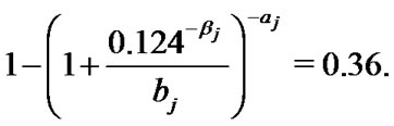
Table 1 shows the values of the hyper-parameters and posterior probabilities obtained for each .
.
By using the algorithm A and the entries of Table 1, the bootstrap estimate, the ML estimate and the Bayes estimates of ,
,  , and
, and  are presented in Table 2.
By using the real data of lower record values in Algorithm A the confidence intervals of ,
,  , and
, and  are presented in Table 3.
6.2. Progressive Type II Censored
Example 2. (Real data) We will take the same values in

Table 1. Prior information, hyper-parameters and the posterior probabilities.
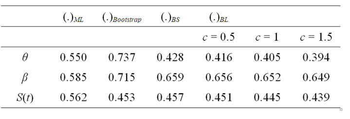
Table 2. The ML, Bayes and bootstrap estimates of θ, β and S(t) with t = 0.5 and ω = 0.2.
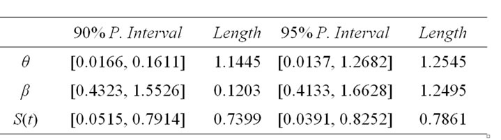
Table 3. Two-sided 90% and 95% confidence intervals of θ, β and S(t) by bootstrap estimate.
example 1.
0.013; 0.027; 0.029; 0.0307; 0.0314; 0.082; 0.121; 0.124; 0.136; 0.154; 0.21; 0.214; 0.24; 0.32;0.36; 0.76; 1.04; 1.28; 5.26. This data have come from the Inverse Wiebull distribution then the MLEs of  and
and , using a Newton-Raphson method are obtained as
  = 0.635814 and
  = 0.825806, so
  = 0.620716, at t = 0.6.
We will use the expected value of  to find the values of the hyper-parameters
  and
and  for Known
 ,
, .
.

These two prior probabilities are substituted into (46), where  and
and  are solved numerically for each given
 ,
,  using Newton-Raphson methods (in Table 4).
Table 5 shows the values of the hyper-parameters and posterior probabilities obtained for each .
.
By using the algorithm A and the entries of Table 5, the bootstrap estimate, the ML estimate and the Bayes estimates of ,
,  , and
, and  are presented in Table 6.

Table 4. Progressive type II censored sample (m = 8, n = 9) from Nelson (1982).

Table 5. Prior information and posterior probabilities.
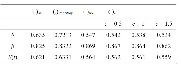
Table 6. The ML, Bayes and bootstrap estimates of θ, β and S(t) with t = 0.6 and ω = 0.2.

Table 7. Two-sided 90% and 95% confidence intervals of θ, β and S(t) by bootstrap estimate.
By using the real data of progressive type II censored sample in Algorithm A the confidence intervals of ,
,  , and
, and  are presented in Table 7.
REFERENCES
- U. Kamps, “A concept of Generalized Order Statistics,” Teubner Stuttgart, 1995,
- U. Kamps and E. Cramer, “On Distributions of Generalized Order Statistics,” Statistics, Vol. 35, No. 3, 2001, pp. 269-280. doi:10.1080/02331880108802736
- H. A. David, “Order Statistics,” 2nd Edition, Wiley, New York, 1981.
- E. Castillo, “Extreme Value Theory in Engineering,” Academic Press, Boston, 1988.
- B. C. Arnold, N. Balakrishnan and H. N. Nagaraja, “A First Course in Order Statistics,” Wiley, New York, 1992.
- E. Cramer and U. Kamps, “Sequential Order Statistics and k-Out-of-n Systems with Sequentially Adjusted Failure Rates,” Annals of Institute of Statistical Mathematics, Vol. 48, No. 3, 1996, pp. 535-549. doi:10.1007/BF00050853
- E. Cramer and U. Kamps, “Marginal Distributions of Sequential and Generalized Order Statistics,” Metrika, Vol. 58, No. 2, 2003, pp. 293-310. doi:10.1007/s001840300268
- V. B. Nevzorov, “Records,” Theory of Probability and Its Applications, Vol. 32, No. 2, 1987, pp. 201-228. doi:10.1137/1132032
- M. Ahsanullah, “Record Statistics,” Nova Science Publisher, Inc., Commack, New York, 1995.
- A. A. Soliman and G. R. Elkahlout, “Bayes Estimation of the Logistic Distribution Based on Progressively Censored Samples,” Journal of Applied Statistical Science, Vol. 14, 2005, pp. 281-293.
- A. A. Soliman, “Estimation of Parameters of Life from Progressively Censored Data Using Burr-XII Model,” IEEE Trans. Reliab, Vol. 54, No. 1, 2005, pp. 34-42. doi:10.1109/TR.2004.842528
- A. A. Soliman, “Estimations for Pareto Model Using General Progressive Censored Data and Asymmetric Loss,” Communications in Statistics Theory & Methods, Vol. 37, No. 9, 2008, pp. 1353-1370. doi:10.1080/03610920701825957
- A. A., Soliman, A. H. Abd Ellah, N. A. Abou-Elheggag and A. A. Modhesh, “Bayesian Inference and Prediction of Burr Type XII Distribution for Progressive First Failure Censored Sampling,” Intelligent Information Management, Vol. 3, 2011, pp. 175-185.
- N. Balakrishnan and A. Asgharzadeh, “Inference for the Scaled Half-Logistic Distribution Based on Progressively Type-II Censored Samples,” Communications in Statistics Theory & Methods, Vol. 34 , No. 1, 2005, pp. 73-87.
- A. M. Sarhan and A. Abuammoh, “Statistical Inference Using Progressively Type-II Censored Data with Random Scheme,” Int. Math. Forum, Vol. 3, No. 33-36, 2008, pp. 1713-1725.
- A. S. Wahed, “Bayesian Inference Using Burr Model Under Asymmetric Loss Function: An Application to Carcinoma Survival Data,” Journal of Statistical Research, Vol. 40, No. 1, 2006, pp. 45-57.
- J. R. Alicja, “A Sequential Estimation Procedure for the Parameter of an Exponential Distribution under Asymmetric Loss Function,” Statistics & Probability Letters, Vol. 78, No. 17, 2008, pp. 3091-3095.
- A. H. Abd Ellah, “Bayesian Prediction of Weibull Distributions Based on Fixed and Random Sample Size,” Serdica Mathematical Journal, Vol. 35, 2009, pp. 129- 146.
- A. H. Abd Ellah, “Parametric Prediction Limit for Generalized Exponential Distribution Using Record Observations,” Applied Mathematics & Information Science, No. 2, 2008, pp. 135-149.
- A. H. Abd Ellah, “Comparison of Estimates Using Record Statistics from Lomax Model: Bayesian and NonBayesian Approaches,” Journal of Statistical Research of Iran Statistical Research and Training Center, Vol. 3, No. 2, 2006, pp. 139-158.
- K. S. Sultan, “Bayesian Estimates Based on Record Values from the Inverse Weibull Lifetime,” Model Quality Technology & Quantitative Management, Vol. 5, No. 4, 2008, pp. 363-374.
- W. B. Nelson, “Applied Life Data Analysis,” John Wiley & Sons, New York, 1982.
- R. Calabria and G. Pulcini, “On the Maximum Likelihood and Least Squares Estimation in the Inverse Weibull Distribution,” Statistica Applicata, Vol. 2, No. 1, 1990, pp. 53-66.
- M. Maswadah, “Conditional Confidence Interval Estimation for the Inverse Weibull Distribution Based on Censored Generalized Order Statistics,” Journal of Statistical Computation and Simulation, Vol. 73, No. 12, 2003, pp. 887-898. doi:10.1080/0094965031000099140
- R. Dumonceaux and C. E. Antle, “Discrimination between the Lognormal and Weibull Distribution,” Technometrics, Vol. 15, 1973, pp. 923-926. doi:10.2307/1267401
- D. N. P. Murthy, M. Xie and R. Jiang, “Weibull Model,” John Wiley & Sons, New York, 2004.
- J. Ahmadi, M. J. Jozani, E. Marchand and A. Parsian, “Bayes Estimation Based on k-Record Data from a General Class of Distributions under Balanced Type Loss Functions,” Journal of Statistical Planning and Inference, Vol. 139, No. 3, 2009, pp. 1180-1189.
- J. F. Lawless, “Statistical Models and Methods for Lifetime Data,” John Wiley & Sons, New York, 2003.
- R. Aggarwala and N. Balakrishnan, “Maximum Likelihood Estimation of Laplace Parameters Based on Progressive Type-II Censored Samples,” In: N. Balakrishnan, Ed., Advances in Methods and Applications of Probability and Statistics, Gordon & Breach Publishers, New York, 1999.
- H. K. T. Ng, P. S. Chan and N. Balakrishnan, “Optimal Progressive Censoring Plans for the Weibull Distribution,” Technometics, Vol. 46, No. 4, 2004, pp. 470-481. doi:10.1198/004017004000000482
- N. Balakrishnan, N. Kannan, C. T. Lin and H. K. T. Ng, “Point and Interval Estimation for Gaussian Distribution Based on Progressively Type-II Censored Samples,” IEEE Transactions on Reliability, Vol. 52, No. 1, 2003, pp. 90-95. doi:10.1109/TR.2002.805786
- N. Balakrishnan, “Progressive Censoring Methodology: An Appraisal,” Test, Vol. 16, No. 2, 2007, pp. 211-259. doi:10.1007/s11749-007-0061-y
- N. Balakrishnan and R. A. Sandhu, “A Simple Simulational Algorithm for Generating Progressive Type-II Censored Samples,” American Statistician, Vol. 49, No. 2, 1995, pp. 229-230. doi:10.2307/2684646
- B. C. Arnold, N. Balakrishnan and H. N. Nagaraja, “Record,” Wiley, New York, 1998.
- B. C. Arnold and S. J. Press, “Bayesian Estimation and Prediction for Pareto Data,” Journal of the Acoustical Society of America (JASA), Vol. 84, 1998, pp. 1079-1084.
- M. Burkschat, E. Cramer and U. Kamps, “Linear Estimation of Location and Scale Parameters Based on Generalized Order Statistics from Generalized Pareto Distributions,” In: M. Ahsanullah, Ed., Recent Developments in Ordered Random Variables, Nova Science Publisher, New York, 2007, pp. 253-261.
- R. M. Soland, “Bayesian Analysis of the Weibull Process with Unknown Scale and Shape Parameters,” IEEE Transactions on Reliability, Vol. R18, No. 4, 1969, pp. 181- 184. doi:10.1109/TR.1969.5216348
- B. Efron, “Censored Data and Bootstrap,” Journal of the American Statistical Association, Vol. 76, No. 374, 1981, pp. 312-319. doi:10.2307/2287832
- B. Efron and R. J. Tibshirani, “Bootstrap Method for Standard Errors, Confidence Intervals and Other Measures of Statistical Accuracy,” Statistical Science, Vol. 1, No. 1, 1986, pp. 54-75. doi:10.1214/ss/1177013815
- H. F. Martz and R. A. Waller, “Bayesian Reliability Analysis,” John Wiley & Sons, New York, 1982.