Positioning
Vol.4 No.1(2013), Article ID:28338,7 pages DOI:10.4236/pos.2013.41001
Monitoring Bridge Deformation Using Auto-Correlation Adjustment Technique for Total Station Observations
![]()
Public Works and Civil Engineering Department, Faculty of Engineering, Mansoura University, Mansoura, Egypt.
Email: ashraf.beshr@gmail.com, mosbeh.kaloop@gmail.com
Received December 9th, 2012; revised January 10th, 2013; accepted January 29th, 2013
Keywords: Monitoring; Total Station; Auto-Correlation; Bridges; Deformation
ABSTRACT
Bridges are omnipresent in every society and they affect its human, social, ecological, economical and cultural aspects. This is why a durable and safe usage of bridges is an imperative goal of structural management. Measurement and monitoring have an essential role in structural management. The benefits of the information obtained by monitoring are apparent in several domains. In deformation analysis, the functional relationship between the acting forces and the resulting deformations should be established. If time depending observations are given, a regression could be used as a functional model. In case of stochastic model, uncorrelated observations with identical variance are assumed. Due to the high sampling rate, a small time difference arises between two observations. Thus the assumed stochastic model is not suitable. The calculation has to be effected by means of auto-correlated observations. This paper investigates an integrated monitoring system for the estimation of the deformation (i.e., static, quasi-static) behavior of bridges from total station observations and studies the effect of autocorrelation technique on the accuracy of the estimated parameters and variances. The results have shown that autocorrelation technique is reduced the standard deviation of X&Y-direction about 6.7% to 29.4% and 6.5% to 15.5% of the original value, respectively, but the situation was differ in Z direction; the standard deviation in vertical component Z was increased.
1. Introduction
In order to know the safety of bridges, monitoring their real-time displacement and recording their fatigue history are very important. The methods, which are often used for such survey, are acceleration integration method and laser distance gauge method. The acceleration integration method integrates the acceleration, which is measured by acceleration gauge, to obtain the displacement. But its error is relatively large. The laser distance gauge method is often influenced by the weather [1-3]. Furthermore, the application of using the two mentioned methods often needs to stop the traffic, which brings a lot of costs. So these methods are suitable for some structures whose survey distance is relatively short and the displacement is relatively small. But for other structures like effective bridges, these methods are difficult to use.
With the development of motorized and reflectorless total station and least square adjustment by computer programs, the monitoring of deformation becomes more available and accurate. At present, total station has been widely spread and used in many survey sites, and sometimes it is not fully used since users misunderstand the principles of this unit [1,4,5-8]. It should be intuitive that deformation monitoring technique will vary according to the type of structure. So a flexible surveying monitoring method and resulted data adjustment technique are needed to monitor the structural deformation of special structures like bridges and make the process of measurements easier and accurate.
In many continuous deformation monitoring process, data (observations) are obtained sequentially using motorized total station. Sometimes relationships exist in the sequential data. Just as the sample correlation coefficient may be used to characterize the relationship between the measured parameters, the autocorrelation coefficient may be used to characterize relationships between observations in the same sequence of values.
Autocorrelation is the cross-correlation of a signal with itself. Informally, it is the similarity between observations as a function of the time separation between them. It is often used in signal processing for analyzing functions or series of values, such as time domain signals [9- 12]. In addition, the statistical autocorrelation of a random process describes the correlation between values of the process at different times, as a function of the two times or of the time difference [7,9,11].
This paper presents observations technique for monitoring the bridge deformation and studies the availability of applying auto-correlation adjustment technique for total station observations.
2. Mathematical Model and Auto-Correlation Technique
This section presents the pre-analysis study of the suggested monitoring technique for monitoring the bridge performance such as displacement, strain, vibration, settlement and rotation. The intersection process in three dimensions using the two total stations technique is used for monitoring the deformation of bridge. This model employed the intersection in three dimensions to determine the spatial coordinates of a specific target on the monitored structure. Figure 1 illustrates the geometry of the two total stations technique.
A local three-dimensional rectangular coordinates system is needed to calculate the spatial coordinates of any target points. Such a system, presumably, has X-axis is chosen as a horizontal line parallel to the base direction, which Y-axis is a horizontal line perpendicular to the base direction and positive in the direction towards the object, Z-axis is a vertical line determined by the vertical axis of the instrument at occupied station. There are two known coordinates points (XA, YA, ZA) and (XC, YC, ZC). From these two known points (A and C), we can determine the coordinates of unknown point B.
From Figure 1, there are three unknowns (XB, YB, ZB) and six observations (two slope distances S1, S2, two horizontal angles α1, α2, and two vertical angles γ1, γ2). The unconditional least squares method, which minimizes the error sum of squares for all observations, will be used to get the most probable value of unknowns. In this model of adjustment, the number of equations is equal to the number of observations (n = 6).
The two lengths of the lines  in the space can be written as:
 (1)
(1)
By using the coordinates formulae, the two lines AB and CD in the horizontal projection can be written as follows:
 (2)
(2)
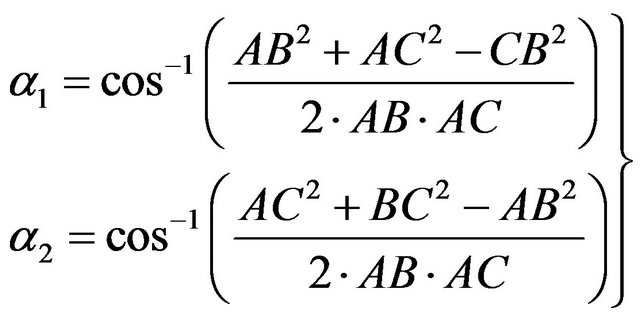
From Figure 1, the horizontal angles (α1 and α2) can be calculated as follows:
 (3)
(3)
By using the coordinates formulae, the Equation (3) can be written as:

Figure 1. The geometry of two total stations technique.
 (4)
(4)
The vertical angles (γ1 and γ2) can be calculated as following:
 5))
5))
The Equations (1), (4) and (5) are the six observational equations, these equations are nonlinear function of both parameters and observations; they can be treated by least squares adjustment technique.
In this model uncorrelated total station observations are assumed, then the weight matrix of observations can be calculated which has dimensions (6 × 6). So, the coordinates of each point on the monitored structure will be calculated and their standard deviations.
Regression analyses that do not compensate for spatial dependency can have unstable parameter estimates and yield unreliable significance tests. Spatial regression models capture these relationships and do not suffer from these weaknesses. It is also appropriate to view spatial dependency as a source of information rather than something to be corrected. Spatial dependency leads to the spatial autocorrelation problem in statistics since, like temporal autocorrelation, this violates standard statistical techniques that assume independence among observations. So the calculation of monitoring points coordinates has to be affected by means of auto-correlated observations.
The correlation coefficient is a measure of how closely two quantities are related [5,9], it can be calculated as:
 Unit-less (6)
where:
σa: The standard deviation of the first quantity;
σb: The standard deviation of the second quantity;
σab: The covariance of the two quantities;
The correlation coefficient has a limit ±1 [1,8].
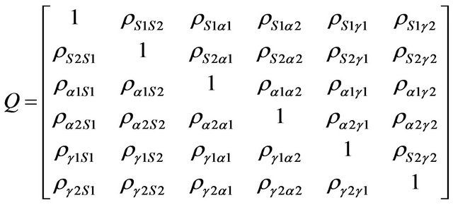
The correlation between neighbored measurements has to be taken into consideration in auto-correlation technique. In this technique, the elements of the cofactor matrix are the correlation coefficients between immediately neighbored values of observations from regression analysis [13]. The symmetrical cofactor matrix (Q) has the (6 × 6) dimensions. In this case, it has the form as following:
 (7)
(7)
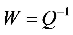
Then, the weight matrix (W) can be calculated as following:
 (8)
(8)
So depending on the variance covariance matrix of observations resulted from regression analysis (observational least square), the new weight matrix will be formed using Equations (7) and (8). This new weight matrix (W) will be reentered in the regression analysis; then the new values of monitoring points coordinates and its standard deviations will be calculated.
3. Description of the Studied Bridge
The bridge has been chosen for the purpose of the deformation monitoring study. The studied bridge is ElDerasat Bridge in Mansoura city-Egypt situated across El-Mansouria channel to connect Mansoura city to the surrounding areas as shown in Figures 2(a) and (b). The bridge has total length 54.5 m and a width 6.85 m; it is made of reinforced concrete and supported on three pillars and two abutments. The monitoring technique involves the following three stages:
1) Site reconnaissance and topographic surveying of the bridge.
2) The actual field measurements by suggested techniques and the documentation of the proposed network stations.
3) The network analysis that deals with the process and analysis of the collected geodetic data.
The bridge is subjected to two types of loads; the first type is static-dead-load, which includes the own weight of the bridge (superstructure and covering materials). The second type is moving-live-loads, these moving
 (a)
(a) (b)
(b)
Figure 2. Topographic surveying of El-derasat bridge (a) Horizontal plan; (b) Vertical plan.
loads due to the transportation on the bridge. Moving loads of vehicles cause impact and dynamic forces, which affect the strength of the bridge.
4. Structural Data Analysis
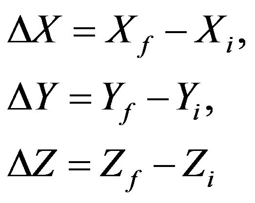
Structural analysis is required to determine whether significant movements are occurred between the monitoring campaigns. Geometric modeling is used to analyze spatial displacements. General movement trends are described using a sufficient number of discrete point displacements  for n stands for the point number, Point displacements are calculated by differencing the adjusted coordinates for the most recent survey campaign (f), from the coordinates obtained at reference time (i), for the stands for the X, Y and Z coordinate displacement, respectively, as following:
 (9)
(9)
Each movement vector has magnitude and direction expressed as point displacement coordinate differences. These vectors describe the displacement field over a given time interval.
The Total Station observations are corrected by least square methods, so this analysis is constrained on the random errors. Comparison of the magnitude of the calculated displacement and its associated accuracy indicates whether the reported movement is more likely due to observations error [8,14,15].
 , Where:
 : The magnitude of the displacement for point n. It can be calculated as:
 (10)
(10)
(en): The maximum dimension of combined 95% confidence ellipse for point (n), it can be calculated as following [15]:
 (11)
(11)
where: σf is the standard error in position for the (final) or most recent survey, σi is the standard error in position for the (initial) or reference survey.
Then, if 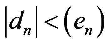 the point isn’t moved. And if
  the point is moved.
5. Observations and Deformation Models
The proposed monitoring network as shown in Figure 3 consists of eleven monitoring surveying points; the spatial distribution of these points should provide complete coverage of the bridge. There are two-bench marks outside the bridge (BM1 and BM2). This system of points is observed from two occupied stations (A and B) by using two total stations techniques. The coordinates of point A are assumed to be (0, 0, 0). The selected monitoring points are located where the maximum deformations have been predicted such points (10, 7, 5, 2) in Figure 3, plus a few points which is depending on previous experience could signal any potential unpredictable behavior such points (11, 9, 8, 6, 4, 3, 1).
All monitoring points are surveyed by using sheet prism of diameter 1 cm fixed on the superstructure of the bridge and two total station (Nikon DTM 850 and Sokiaa SET300, The manufacturer quotes a standard deviation 0.5'' to 1'' for angle measurements and ±(2 + 2 ppm × D) mm for EDM measurements with prisms) fixed at points A and B for two cases of loading (empty and loading cases).
The adjusted coordinates and its associated standard deviations of each point in the monitoring network are calculated by using Matlab program with and without applying auto-correlation adjustment technique. The correlation coefficients between adjusted observations from regression analysis have to be taken into consideration to form the cofactor matrix (Q).
With application of autocorrelation technique, the standard deviations for the first case (empty bridge) are varied from 0.26 mm to 1.09 mm in the horizontal components, and from 4.3 mm to 44.4 mm in vertical component. While in the second case (load bridge), the corresponding values are varied from 0.26 mm to 1.2 mm in horizontal components and from 6.5 mm to 60.3 mm in vertical component. Practically, the overall analysis has shown that the autocorrelation technique improved the accuracy of horizontal components (X and Y directions) but did not improve the vertical component.
The comparison between the resulted standard deviations of the coordinates from regression analysis by using autocorrelation and without autocorrelation can be indicated as shown in Figures 4-6 and Table 1.
As indicated in Figures 4-6 and Table 1, the standard deviation in X direction (σX) was reduced by using autocorrelation technique about 6.7% to 29.4% of the original value—without autocorrelation—the standard deviation in Y direction (σY) was reduced also about 6.5% to 15.5% of the original value but the situation was differ in Z direction, the standard deviation in vertical component Z was increased. The vertical displacement for the studied bridge is much smaller than the confidence in the horizontal displacement, and it therefore does not indicate a significant vertical movement. So, the auto-correlation adjustment technique has a great effect on the decision of the monitoring point movement.
6. Conclusions
The results of experimental work lead to the following conclusions:
1) The proposed surveying techniques (two total stations which employed the intersection process) can provide valuable data on the deformation of the structural members and movement of buildings.
2) Auto-correlation adjustment technique depends mainly on the variance covariance matrix of observations, it improves the standard deviation in horizontal plane (X
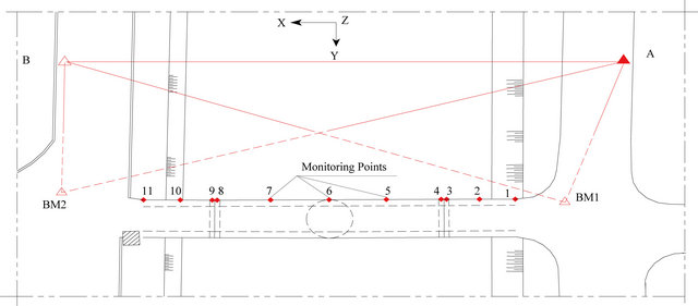
Figure 3. System of observation for bridge monitoring.
Table 1. Comparison between regression analysis with and without auto-correlation technique.
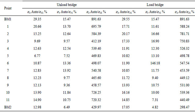
σX Auto, σY Auto and σZ Auto are the standard deviation in X, Y and Z direction with autocorrelation technique respectively. σX1, σY1 and σZ1 are the standard deviation in X, Y and Z direction without autocorrelation technique respectively.
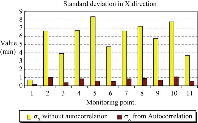
Figure 4. Comparison between regression analysis with and without Auto-Correlation for σX.

Figure 5. Comparison between regression analysis with and without Auto-Correlation for σY.
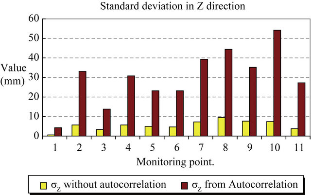
Figure 6. Comparison between regression analysis with and without Auto-Correlation for σZ.
and Y), but it has a bad effect on vertical direction (Z).
3) Achieving the required accuracy for surveying monitoring technique is based on the following factors:
a) The used instruments specifications (Instrument resolution, data collection options and the proper operating instructions).
b) The field observation and modeling procedures. Measurements and adjustment techniques of the network have direct influence on the detection of monitoring point’s displacements.
7. Acknowledgements
The authors are supported from Faculty of Engineering, Mansoura University.
REFERENCES
- A. Beshr, “Accurate Surveying Measurements for Smart Structural Members,” M.S. Thesis, Mansoura University, El-Mansoura, 2004.
- G. Roberts, E. Cosser, X. Meng, A. Dodson, A. Morris and M. Meo, “A Remote Bridge Health Monitoring System Using Computational Simulation and Single Frequency GPS Data,” Proceedings of 11th FIG Symposium on Deformation Measurements, Santorini, 25-28 May 2003.
- V. Gikas, “Ambient Vibration Monitoring of Slender Structures by Microwave Interferometer Remote Sensing,” Journal of Applied Geodesy, Vol. 6, No. 3-4, 2012, pp. 167-176. doi:10.1515/jag-2012-0029
- D. Li, “Sensor Placement Methods and Evaluation Criteria in Structural Health Monitoring,” Ph.D. Thesis, Universität Siegen, Siegen, 2011.
- S. Stiros and P. Psimoulis, “Response of a Historical Short-Span Railway Bridge to Passing Trails: 3-D Deflections and Dominant Frequencies Derived from Robotic Total Station (RTS) Measurements,” Engineering Structures, Vol. 45, 2012, pp. 362-371. doi:10.1016/j.engstruct.2012.06.029
- V. Zarikas, V. Gikas and C. P. Kitsos, “Evaluation of the Optimal Design ‘Cosinor Model’ for Enhancing the Potential of Robotic Theodolite Kinematic Observations,” Measurement, Vol. 43, No. 10, 2010, pp. 1416-1424. doi:10.1016/j.measurement.2010.08.006
- M. Kaloop, A. Beshr and M. Elshiekh, “Using Total Station for Monitoring the Deformation of High Strength Concrete Beams,” 6th International Conference on Vibration Engineering (ICVE’2008), Dalian, 4-6 June 2008, pp. 411-419.
- A. Beshr, “Monitoring the Structural Deformation of Tanks,” Lambert Academic Publication, Germany, 2012.
- N. Elsheimy, “ENGO 361 Course of Least Square Estimation,” University of Calgary, Calgary, 2001.
- M. Kaloop, “Bridge Safety Monitoring Based-GPS Technique: Case Study Zhujiang Huangpu Bridge,” Smart Structures and Systems, Vol. 9, No. 6, 2012, pp. 473-487.
- E. Mikhail and G. Gracie, “Analysis and Adjustment of Survey Measurements,” Van Nostrand Reinhold Company, New York, 1981.
- P. Stella, A. Villy and C. S. tathis, “Analysis of the Geodetic Monitoring Record of the Ladhon Dam,” FIG Working Week, Athens, 22-27 May 2004.
- H. Kuhlmann, “Importance of Autocorrelation for Parameter Estimation in Regression Models,” The 10th FIG International Symposium on Deformation Measurements, Orange, 19-22 March 2001.
- SPSS. Inc., “Version 10.0.5,” Chicago, 1999.
- J. Schroedel, “Engineering and Design Structure Deformation Surveying,” CECWEE Manual No. 1110-2-1009, Department of the Army, US Army Crops of Engineering, Washington DC, 2002.

