Positioning
Vol.2 No.4(2011), Article ID:8313,10 pages DOI:10.4236/pos.2011.24013
Error Analysis of Orbit Determination for the Geostationary Satellite with Single Station Antenna Tracking Data
![]()
Aeronautics and Astronautics Faculty, Istanbul Technical University, Istanbul, Turkey.
Email: cingiz@itu.edu.tr
Received July 21st, 2011; revised August 28th, 2011; accepted September 22nd, 2011.
Keywords: Orbit Determination, Geostationary Satellite, Single Station Antenna, Error Analysis
ABSTRACT
In the study, position and velocity values of a geostationary satellite are found. When performing this, a MATLAB algorithm is used for Runge-Kutta Fehlberg orbit integration method to solve spacecraft’s position and velocity. Integrated method is the solution for the systems which mainly work with a single station. Method provides calculation of azimuth, elevation and range data by using the position simulation results found by RKF. Errors of orbit determination are analysed. Variances of orbit parameters are chosen as the accuracy criteria. Analysis results are the indicator of the method’s accuracy
1. Introduction
Orbit determination accuracy improvement for geostationary satellite with single station antenna tracking data is investigated in [1]. In this study, an operational orbit determination (OD) and system for the geostationary satellite (Communication, Ocean and Meteorological Satellite (COMS)) mission requires accurate satellite positioning data to accomplish image navigation registration on the ground. Ranging and tracking data, which is provided by a single ground station, is used to determine the orbit of geostationary satellite in normal operation. However, the orbital longitude of geostationary satellite is so close to that of satellite tracking sites that geometric singularity affects observability [2]. Applying an estimated azimuth bias using the ranging and tracking data provided by two stations is a method to solve the azimuth bias of a single station in singularity. Velocity increments of a wheel offloading maneuver, which is performed twice a day, are fixed by planned values without considering maneuver efficiency during OD. Using only single-station data with the correction of the azimuth bias, OD is succeed to achieve three-sigma position accuracy on the order of 1.5 km root-sum square.
In [3] comparison of Extended Kalman Filter (EKF) and Unscented Kalman Filter (UKF) for spacecraft localization via angle measurements [3] is performed. In the study, performances of two nonlinear estimators are compared for the localization of a spacecraft. It is assumed that range measurements are not available, and the localization problem is tackled on the basis of angle-only measurements. A dynamic model of the spacecraft accounting for several perturbing effects, such as Earth and Moon gravitational field asymmetry and errors associated with the Moon ephemerides, is employed. The measurement process is based on elevation and azimuth of Moon and Earth with respect to the spacecraft reference system. Position and velocity of the spacecraft are estimated using both the extended Kalman filter (EKF) and the unscented Kalman filter (UKF). The behaviour of the filters is compared on two sample missions: Earth-to-Moon transfer and geostationary orbit raising.
Localization of spacecraft is usually very accurate when GPS measurements are available [4]. The problem becomes more challenging when GPS signals are not available, like in high-Earth orbits or in long range missions such as Earth-to-Moon transfers. In these cases spacecraft navigation is often handled by ground-based tracking stations, thus making it unfeasible for low-cost spacecraft missions. In order to make spacecraft fully autonomous, it is necessary to devise self-localization and navigation algorithms relying on measurements provided by onboard sensors. In the study, the problem of spacecraft self-localization is addressed using angular measurements. First a dynamic model of the spacecraft is formulated, which takes into account several perturbing effects such as Earth and Moon gravitational field asymmetry and errors associated with the Moon ephemerides. It is assumed that the navigation system is able to estimate the spacecraft attitude (by using a star tracker sensor), and the spacecraft is equipped with line-of-sight sensors providing measurements of elevation and azimuth of Moon and Earth with respect to the spacecraft reference system. Range measurements, which are often difficult to obtain or are not sufficiently reliable, are not required. Then, position and velocity of the spacecraft are estimated by employing both the classical extended Kalman filter and the recently developed unscented Kalman filter [5]. Comparisons between EKF and UKF have been proposed in several contexts, ranging from target tracking [6], to positioning systems and virtual reality. The filters have been tested on simulated data concerning two different missions. The resulting localization errors [7] and the associated confidence intervals show that the proposed algorithms provide reliable estimates, whose accuracy is sufficient for autonomous navigation in the considered class of missions. In general, for the orbit determination purpose the Kalman filtering technique is used. Accuracy of the Kalman filter depends on the accuracy of the measurement devices significantly. Therefore, it is important to investigate the improvement of the accuracy of measurement instruments.
In the study, a geostationary satellite’s orbit is determined and error analysis of the orbit determination is performed. Runge-Kutta Fehlberg Orbit Integration Method is applied to equation of motion of a satellite. Position and velocity equations are provided via RKF application. Position and velocity are calculated in 5000 points with 20 seconds time interval between every step. Application of the integrated method to the results is the most important subject of this study. It is necessary to be careful about the transformation of ECI coordinates to topocentric coordinates. This type of transformation is applied because of the Earth’s rotation. When, spacecraft’s position changes at every point, ground station’s coordinates also change due to Earth’s spin. Therefore, ground station’s coordinates are calculated in 5000 points by using sidereal time and latitude. First, satellite’s position is calculated in ECI coordinates. Then, it is transformed to the topocentric coordinates and range, azimuth, elevation angles are calculated. Error and variance can be analyzed after the explained procedure. Variances of the orbit parameters are chosen as the accuracy criteria. Their changes and effects of these changes are investigated.
Study’s operation concept can be defined as (Figure 1).
2. Orbit Integration by Runge-Kutta Fehlberg Method
The equation of motion of a satellite is a second order vector differential equation (see Appendix A).
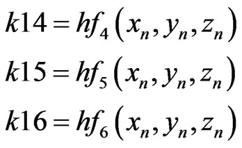
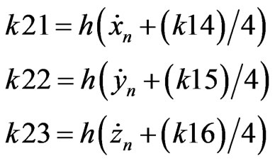
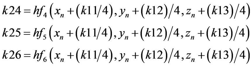
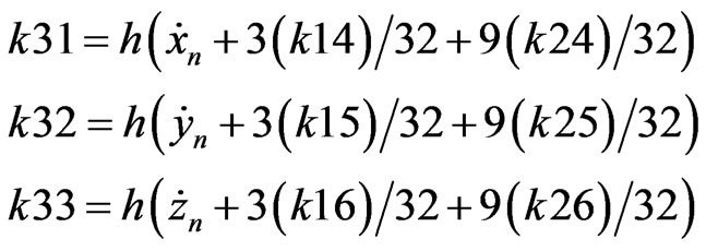
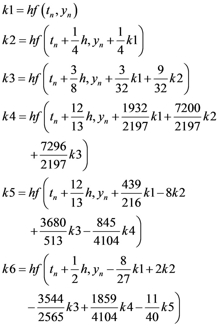
Method can be applied for orbit integration. The solution of first order differential equation system can be obtained according to Babolian (1994) [8]. The following algorithm is very similar to the described algorithm of RKF. However, this algorithm includes many coefficients to be computed. 36 coefficients are calculated in every step of the 5000 iterations.
First, the initial step size h is selected, and then the RKF coefficients (Appendix B., Equation B.4) are calculated via initial conditions [9].
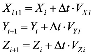
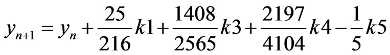
Position and velocity of the satellite are calculated by the following formulas (1), after obtaining the coefficients [9].
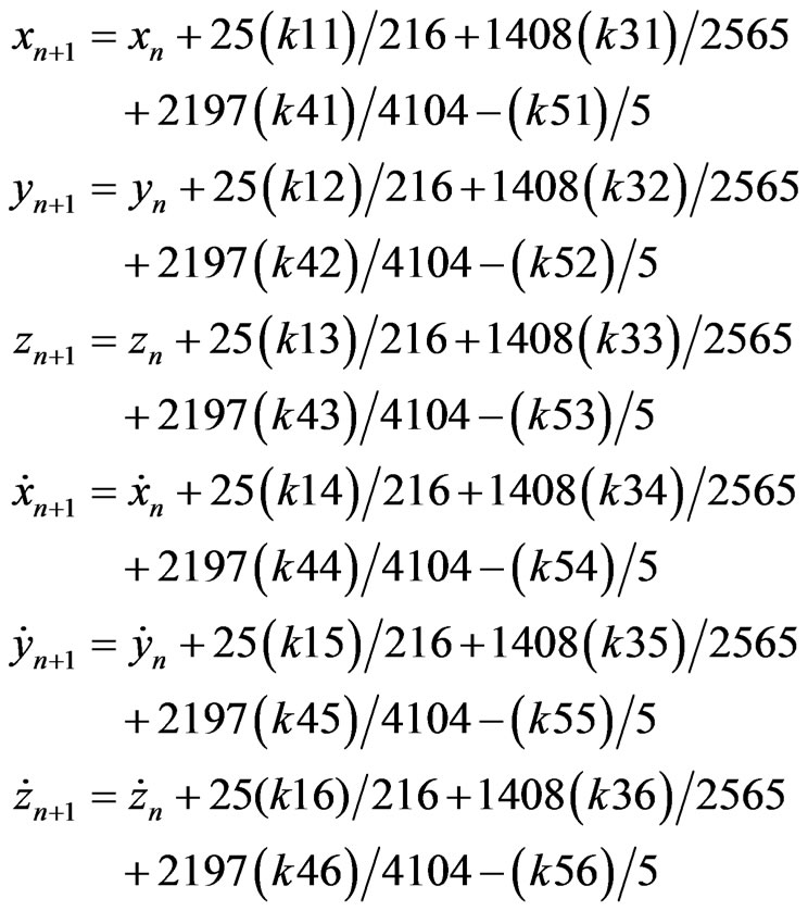 (1)
(1)
3. Determination of the Accuracy of the Spacecraft’s Coordinates
3.1. Determination of the Satellite’s Coordinates by Single Station Antenna Tracking Data
Measurement of angle and measurement of range methods are used at the same time in the integrated method [10]. Integrated method is usually used in radiolocation systems and it determines D range to the satellite, azimuth angle  and elevation angle
 . When this method is used, the coordinates of the satellite is determined as the intersection point of the sphere state surface (D = constant), cone state surface (
 = constant) and vertical plane suitable for
  = constant state surface. Satellite coordinates are determined with single antenna
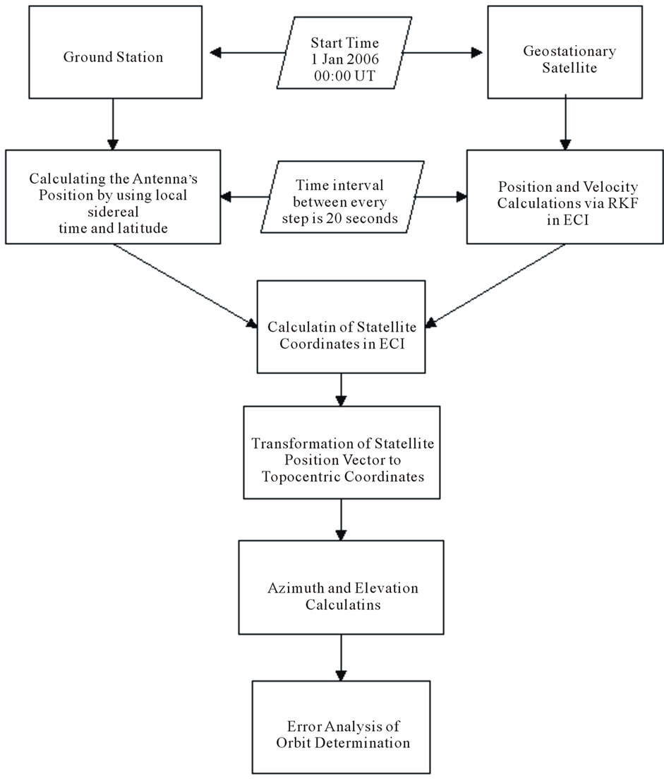
Figure 1. Operation diagram.
(ground station) by integrated method. Method does not need any difficult calculations.
Advantages of the Integrated Method:
• Single station is sufficient to measure the coordinates.
• Coordinates are calculated as simple.
• Method provides the needed accuracy in whole measurement intervals.
• Information processing is easy in system.
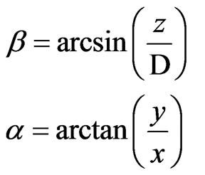
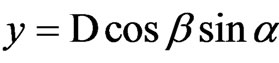
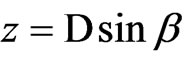
Following formulas are used to calculate satellite coordinates;
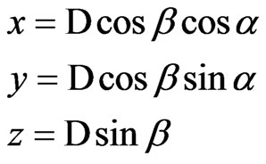 (2)
(2)
where D is the range of the satellite,  is the azimuth angle and
  is the elevation angle, x,y,z are the coordinates of the range between the station and satellite The method is applied to position and velocity calculated by RKF method. The procedure is followed as shown below:
The station must be denoted to satellite vector of the topocentric frame using a coordinate transformation [11,12].
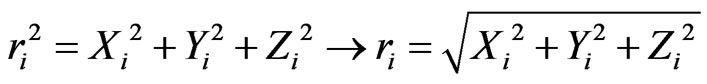
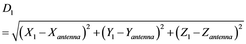
The total range between satellite and ground station;
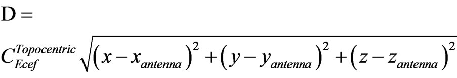 (3)
(3)
where;
 is the transformation matrix from ECEF coordinates to topocentric coordinates.
 is the x coordinate of the antenna’s position.
 is the y coordinate of the antenna’s position.
 is the z coordinate of the antenna’s position.
Calculation of azimuth and elevation angles by total range and range components;
 (4)
(4)
Figures which present range, azimuth and elevation simulations are distributed in Figures 4 and 5.
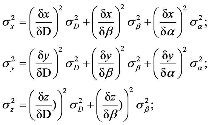
3.2. Variance Analysis of the Satellite’s Coordinates
Characteristics of the position data error depend on the type of ground station, location of ground station, and measurement accuracy of navigation parameters [10]. It is possible to establish ground stations optimally and choose the most accurate region to determine range via necessary calculations. However, calculations are sometimes difficult and some great preparations are necessary. In this case, approximate accuracy values of the coordinates are used to determine the accuracy of range data. Because, x, y, z coordinates of the spacecraft’s range are non-linear function of three parameters measured by angle-range measurement method, the variances of coordinates’ calculation errors are determined as (Equation (5));
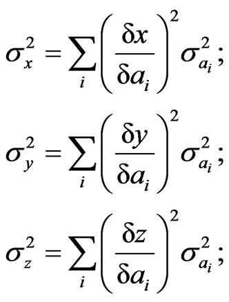 (5)
(5)
where ,
,  and
and  are variances of the calculated coordinates’ errors.
  is the variances of the navigation parameters’ measurement errors.
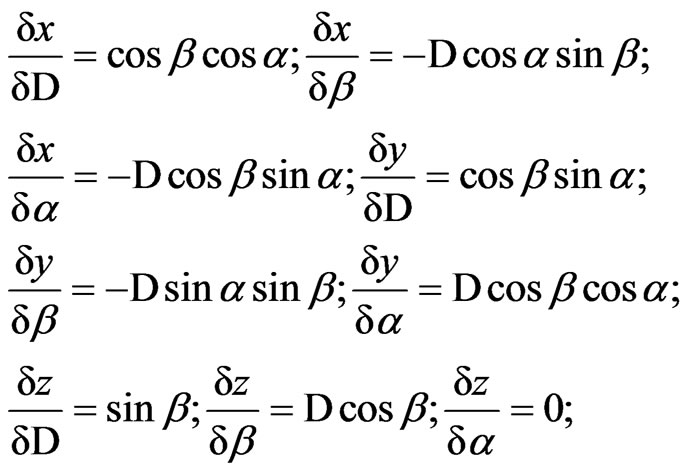
Let’s derive the equations which evaluate the accuracy of the coordinates determined via integrated method [10]. The coordinates of the spacecraft are calculated by formulas;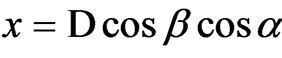 ,
,  ,
,  in this method.
Some equations can be written by assumption of that navigation parameters’ measurement errors are independent;
 (6)
(6)
 ,
,  ,
,  are variances of measurement errors.
 (7)
(7)
Spherical standard deviation is used as the value of the accuracy of spacecraft’s position. It can be written as below;
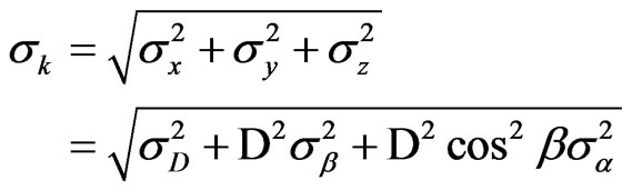 (8)
(8)
4. Simulations
Satellite’s initial position and velocity data are distributed (Table 1). Firstly, satellite’s velocity and position values are calculated in 5000 points. It is done by Runge-Kutta Fehlberg Orbit Integration method. Then, range, azimuth and elevation angle data are obtained via integrated method. Their new values are calculated by addition of some noises and standard deviations. Errors between initial range, azimuth and elevation values and new values are determined and their standard deviation is analyzed. Finally, variance analysis and spherical standard deviations of the results are found and the results are compared. Initial conditions are shown as (Table 1).
Satellite is at 128.2 deg east longitude and the starting time for observation is 1 Jan 2006, 00:00 UT.
Single station antenna which is used for measurements has position data distributed as (Table 2).
1) Simulations for Position and Velocity
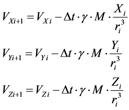
The position and velocity values are calculated in 5000 points (Table 3) with initial conditions in Table 1 and the step size h = 20 by calculating RKF coefficients (Equation B.4). Their simulations are also distributed in Figures 2 and 3.
WhereXrk is the x position coordinate of the satellite.
Yrk is the y position coordinate of the satellite.
Zrk is the z position coordinate of the satellite.
Vxrk is the x velocity coordinate of the satellite.
Vyrk is the y velocity coordinate of the satellite.
Vzrk is the z velocity coordinate of the satellite.
Velocity simulations for x, y and z coordinates are shown in Figure 2.
Position simulations for x, y and z coordinates are shown in Figure 3.
2) Simulations for Azimuth, Elevation and Range
The simulation of the range between spacecraft and antenna is shown in Figure 4.
As it can be seen, range generally decreases up to 2500th step. Then, it shows an increase. For example:
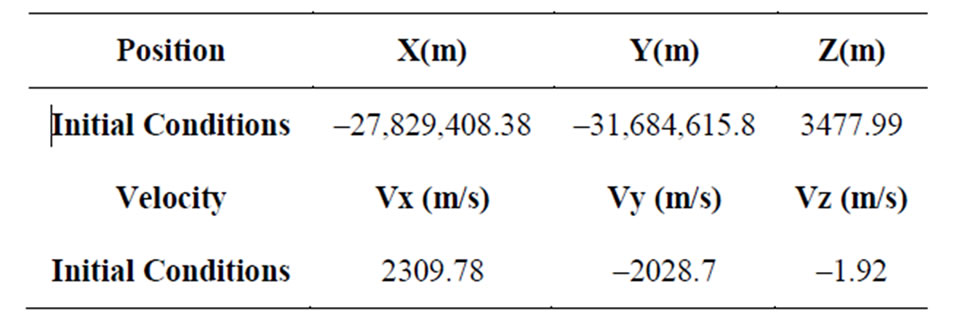
Table 1. Initial position and velocity value.
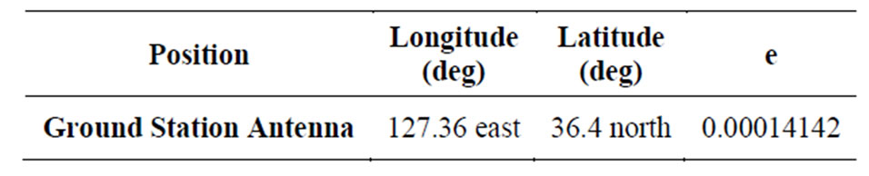
Table 2. Location of ground station.
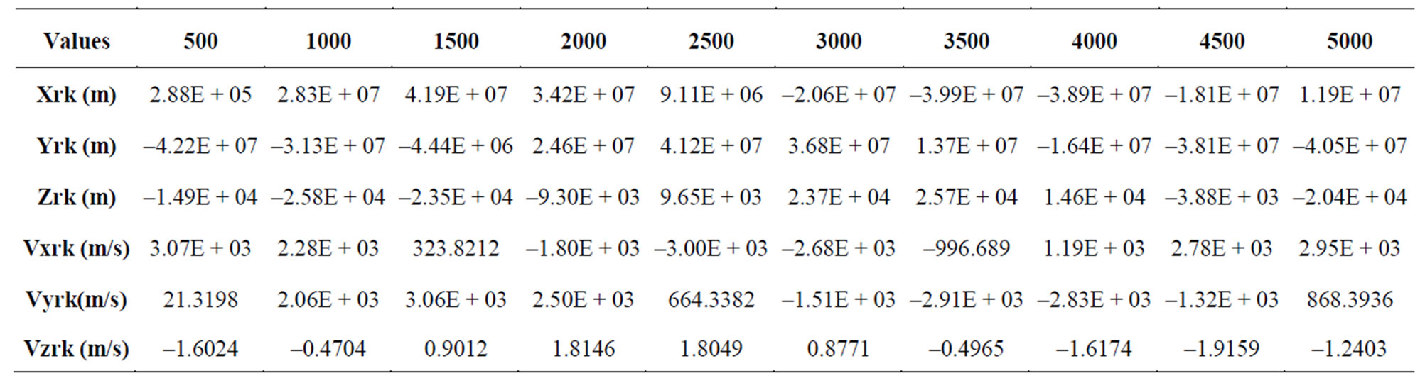
Table 3. Position and velocity values.
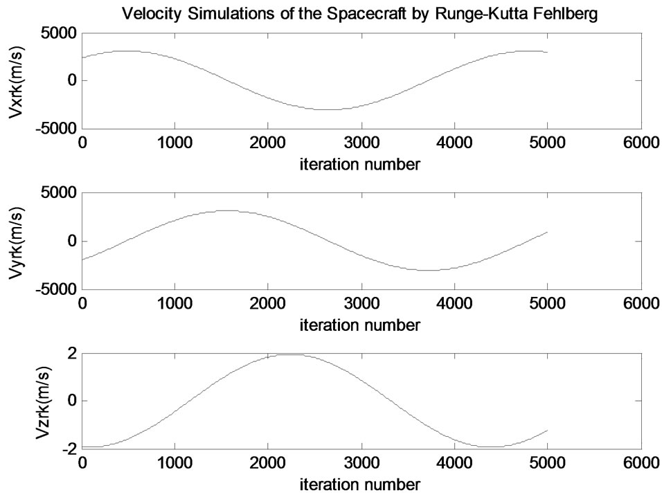
Figure 2. Velocity simulations of the satellite.
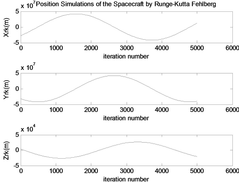
Figure 3. Position simulations of the satellite.
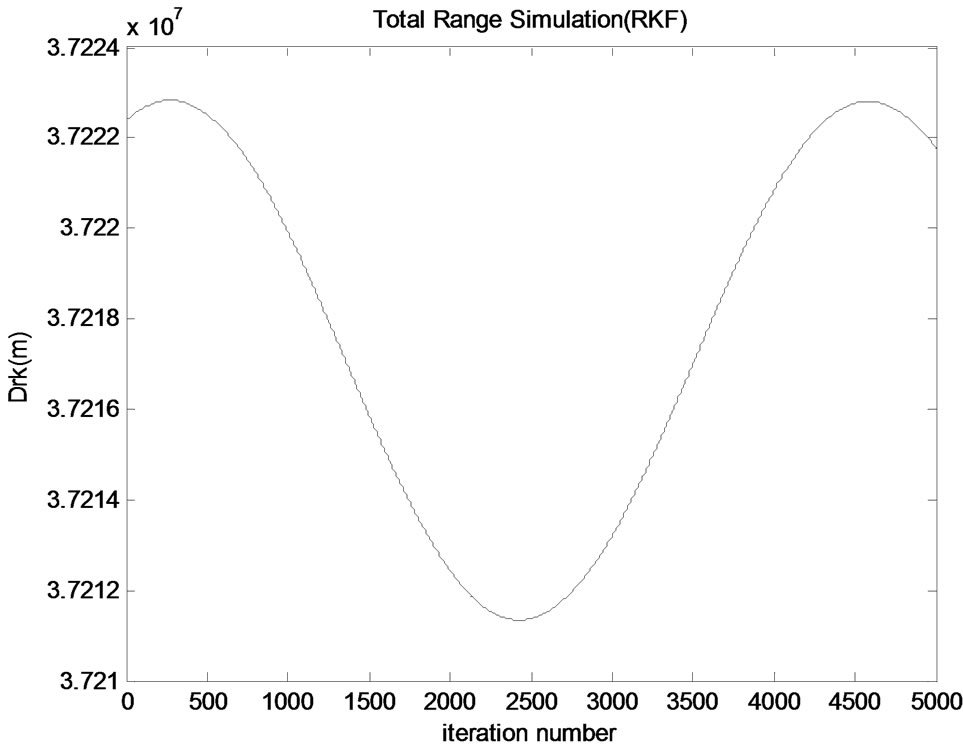
Figure 4. Total range simulation.
think the point which symbolizes the time which is a day later from starting point. This point is between the 4000th - 4500th step interval. If this point is examined, range is nearly the same with the starting point. It can be said that, range is nearly constant for a day period for geostationary satellites.
Simulations for azimuth and elevation angles are shown in Figure 5.
There is a little differentiation from the initial value in both of the angles. These changes are insignificant changes.
3) Simulations for Variance Analysis
The variances, variances components’ analysis and spherical standard deviation results according to integrated method results applied to RKF are shown in Table 4. Their graphics are also shown in Figures 6-10.
The value of the mean spherical standard deviation is 7.83E + 03.
WhereVARxrk is the variance of x position coordinate.
VARyrk is the variance of y position coordinate.
VARzrk is the variance of z position coordinate.
VARxDrk is the variance of x coordinate error due to range uncertainties.
VARxbetark is the variance of x coordinate error due to elevation angle uncertainties.
VARxalfark is the variance of x coordinate error due to azimuth angle uncertainties.
VARyDrk is the variance of y coordinate error due to range uncertainties.
VARybetark is the variance of y coordinate error due to elevation angle uncertainties.
VARyalfark is the variance of y coordinate error due to azimuth angle uncertainties.
VARzDrk is the variance of z coordinate error due to range uncertainties.
VARzbetark is the variance of z coordinate error due to elevation angle uncertainties.
SP.SDEVrk is the spherical standard deviation of the
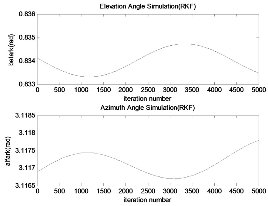
Figure 5. Angles simulation.
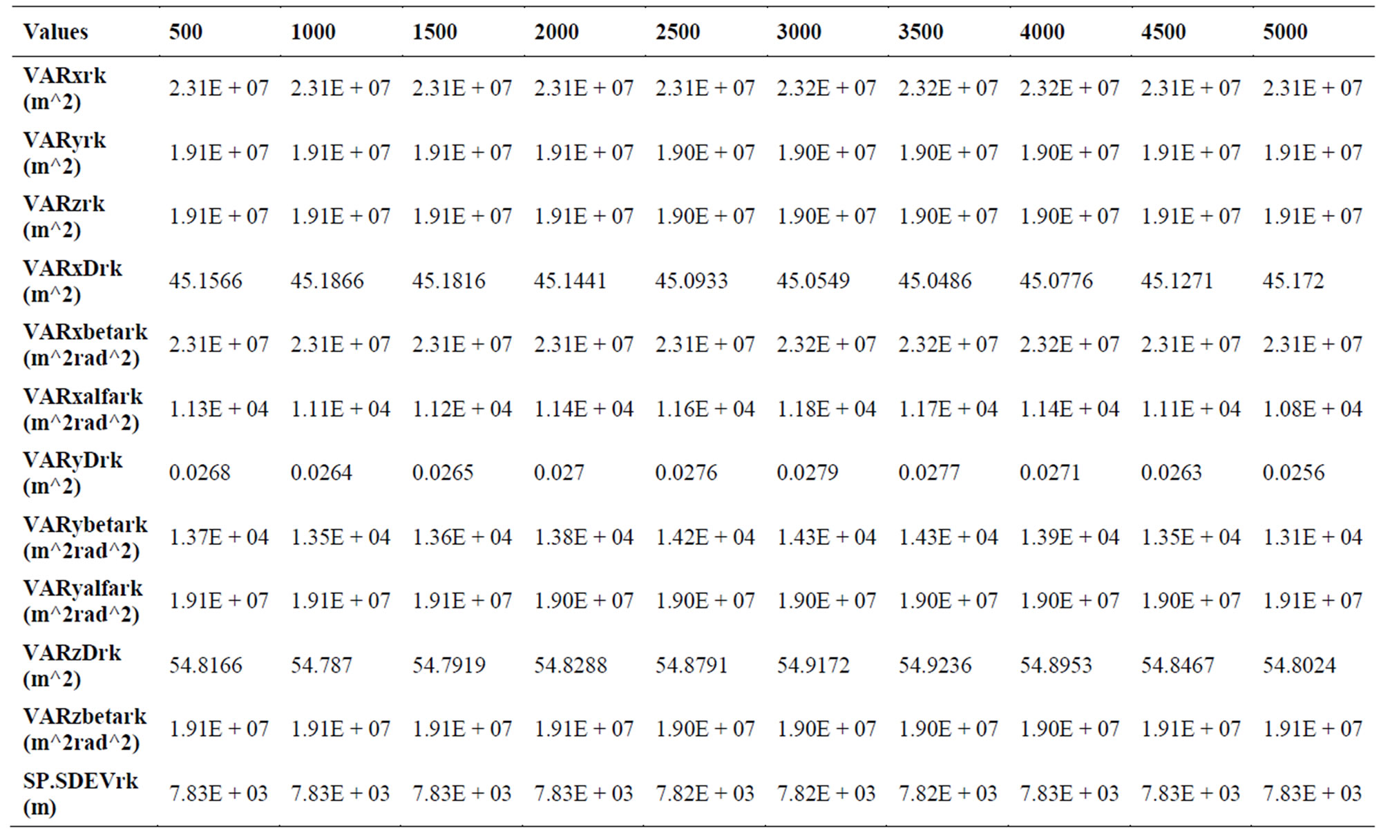
Table 4. Variance analysis.
position.
Variances for x, y and z positions are distributed in Figure 6.
Variances simulations depend on the change of the spacecraft’s position coordinates. Variance changes in only small intervals on orbit operations. As it can be seen, x variance has the biggest value. The biggest amount of change (between peak point and minimum point) is around 10 km for all of the x, y and z variances. Change
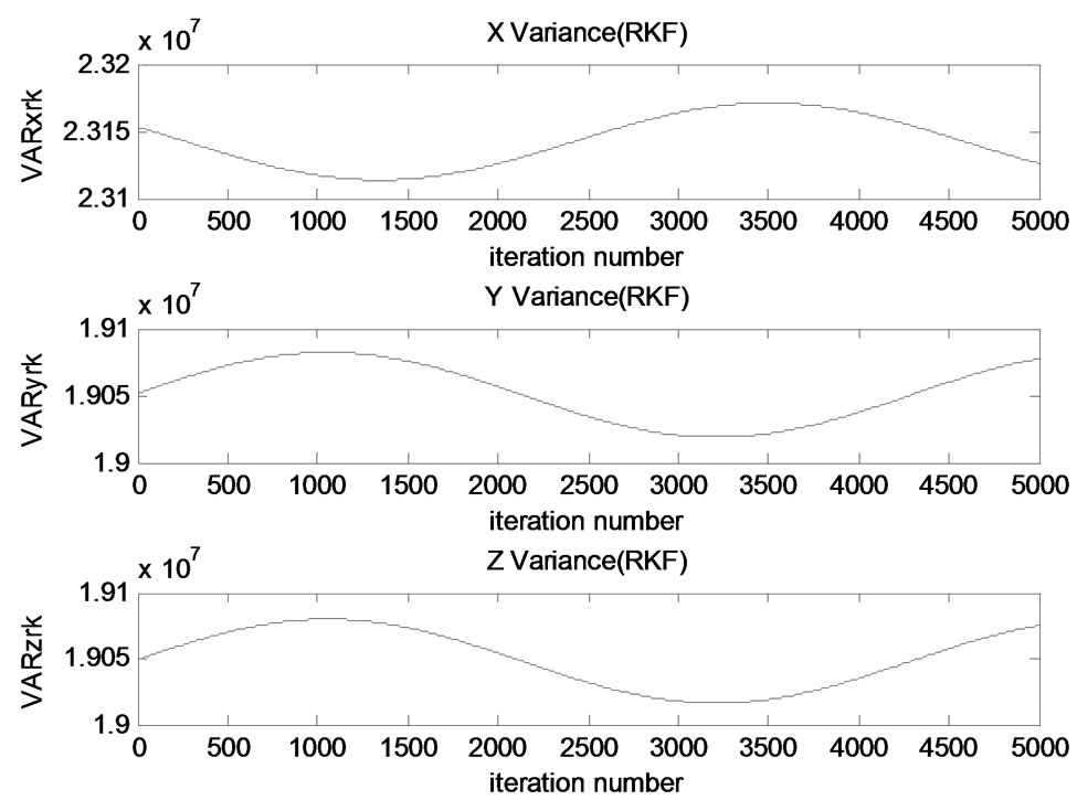
Figure 6. Variances of coordinates x, y, z.
of variances depend on the satellite’s on-orbit action. These changes can take significant values for some parameters such as range, azimuth and elevation. This is an important output since the statistical characteristics of orbit determination errors are generally assumed to be constant.
Components of x coordinate variance are shown in Figure 7.
The components of x, y and z variances are also examined to find how range, azimuth and elevation elements affect the results. It is obvious that elevation angle
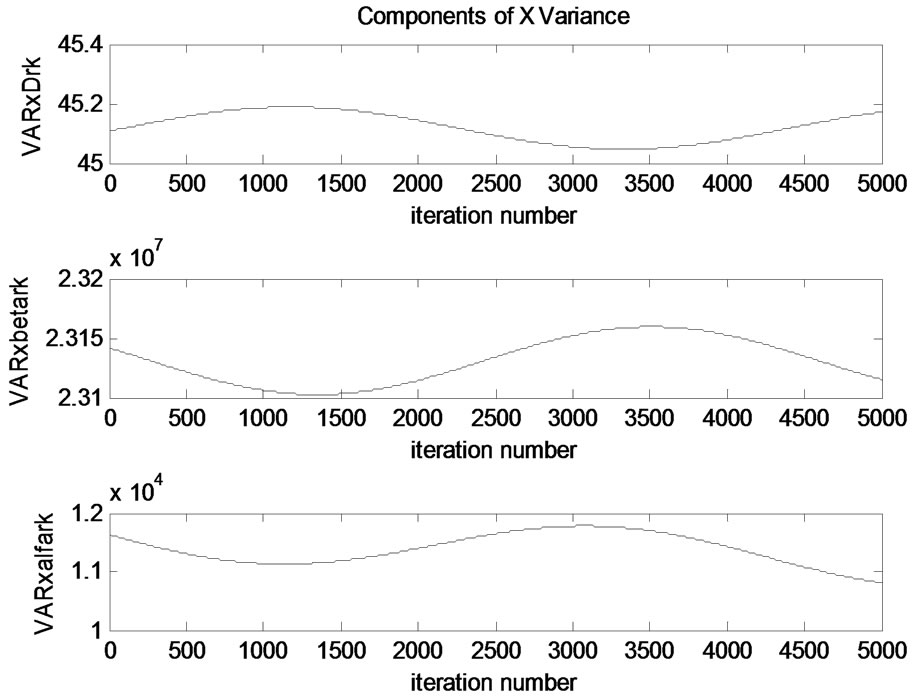
Figure 7. Components of Variance of x coordinate.
affects mostly the X variances. It has higher values than the elevation and range values. Range component has the weakest effect on variation.
Components of y coordinate variance are shown in Figure 8.
Components of Y variance are investigated to understand their effects. Azimuth angle is more dominant in the Y variance. It has higher values than the elevation and range values. Range component has the weakest effect on variation. The components have insignificant variations.
Components of z coordinate variance are shown in Figure 9.
Components of Z variance are investigated to understand their effects. Elevation angle is effective in Z variance. It has higher range value. Z variance components also have some insignificant changes.
Spherical standard deviation of the position is shown in Figure 10.
Spherical standard deviation changes according to the
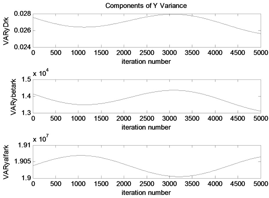
Figure 8. Components of variance of Y coordinate.
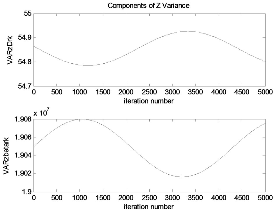
Figure 9. Components of variance of Z coordinate.
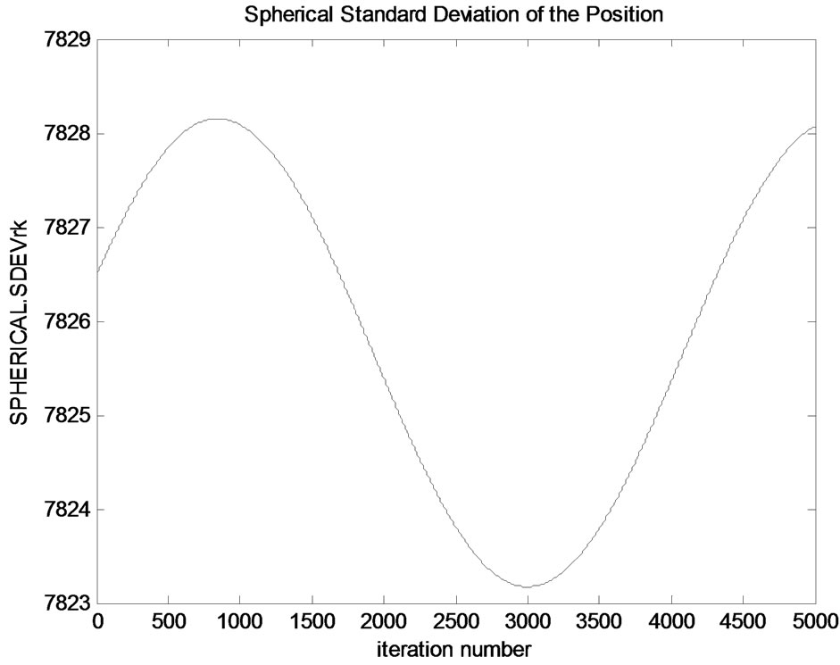
Figure 10. Spherical standard deviation of the satellite position.
spacecraft’s position. It has some insignificant changes. The amount of the biggest change is around 5 meters. It makes a peak around 7828 m and its minimum value is around 7823 meters.
5. Conclusions
In this study, the errors of orbit determination of geostationary satellite with single station antenna tracking data are analyzed. Variances of orbit parameters are chosen as the accuracy criteria. The orbit determination is evaluated via RKF.
Range is nearly constant for a day period of geostationary satellites. There are some small changes when compared with the initial value in azimuth and elevation angles. They changes insignificantly. It can be said that the RKF method gives accurate results by means of logical measurement results for geostationary satellite.
The components of x, y and z variances are also examined to find how range, azimuth and elevation elements affect the results. It is obvious that elevation angle affects mostly the X variances. It has higher values than the elevation and range values. Except elevation, azimuth angle is more dominant in the Y variance. Elevation angle is effective in Z variance. Generally, variances remain nearly constant in results. Range component effect is very small. They have the weakest effects on variations. Spherical standard deviation also shows some insignificant changes. According to very small changes, it can be thought as constant.
REFERENCES
- Y. Hwang, et al., “Orbit Determination Accuracy Improvement for Geostationary Satellite with Single Station Antenna Tracking Data,” ETRI Journal, Vol. 30, No. 6, 2008, pp. 774-782.
- Y. Hwang, et al., “Communication, Ocean, and Meteorological Satellite Orbit Determination Analysis Considering Maneuver Scheme,” AIAA/AAS Astrodynamics Specialist Conference and Exhibit, Keystone, Colorado, August 2006, AAS Paper 2006-6668.
- A. Giannatrapani, et al., “Comparison of EKF and UKF for Spacecraft Localization via Angle Measurements,” IEEE Transactions on Aerospace and Electronic Systems, Vol. 1, No. 47, 2011, pp. 75-84.
- T. Upadhyay, S. Cotterill and A. W. Deaton, “Autonomous GPS/INS Navigation Experiment for Space Transfer Vehicle,” IEEE Transactions on Aerospace and Electronic Systems, Vol. 3, No. 29, 1993, pp. 782-785.
- S. J. Julier and J. K. Uhlmann, “A New Extension of the Kalman Filter to Nonlinear Systems,” The 11th International Symposium on Aerospace/Defence Sensing, Simulation and Controls, Orlando, April 1997, pp. 182-193.
- R. Zhan and J. Wan, “Iterated Unscented Kalman Filter for Passive Target Tracking,” IEEE Transactions on Aerospace and Electronic Systems, Vol. 3, No. 38, 2007, pp. 1155-1163.
- N. Ceccarelli, et al., “Spacecraft Localization via Angle Measurements for Autonomous Navigation in Deep Space,” Proceedings of the 17th IFAC Symposium on Automatic Control in Aerospace, Toulouse, June 2007.
- E. Babolian, “Numerical Methods,” Elm va Sanat University Publication, Department of Mathematics, Theran, 1994.
- M. Es-hagh, “Step Variable Numerical Orbit Integration of a Low Earth Orbiting Satellite,” Journal of the Earth & Space Physics, Vol. 1, No. 31, 2005, pp. 1-12.
- C. Haciyev, “Radyo Navigasyon,” Istanbul Technical University Press, Istanbul, 1999.
- A. Vallado, “Fundamentals of Astrodynamics and Applications,” 2nd Edition, Microcosm Press Jointly with Kluwer Academic Publisher, Torrance, 2001.
- H. D. Curtis, “Orbital Mechanics for Engineering Students,” Elsevier Butterworth-Heinemann, Burlington, 2005.
Appendix A
The Kepler Equations
Kepler equations system is one of the systems which can define elliptic orbits of spacecrafts. This equations system includes 3 equations in differential form:
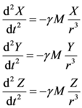 (A.1)
(A.1)
In the equations;
Kepler constant; 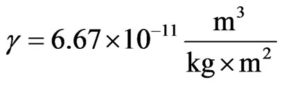
Mass of the Earth; 
Range between spacecraft’s center of mass and earth’s center of mass;
Cartesian coordinates of the spacecraft; 
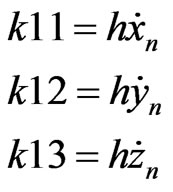
Write the equations in type of the first order differential equations as;
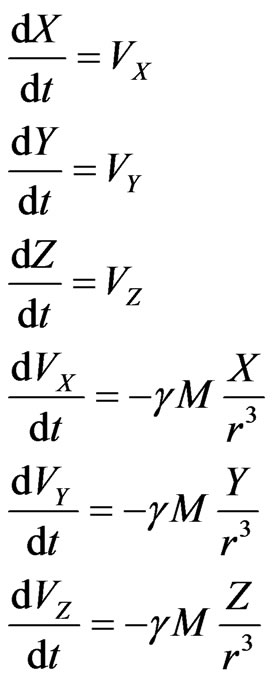 (A.2)
(A.2)
After that, 6 equations are obtained; (A.3-A.4)
 (A.3)
(A.3)
 (A.4)
(A.4)
The range between spacecraft and ground station;
 (A.5)
(A.5)
Appendix B
Runge-Kutta Fehlberg Integration Method
The Runge-Kutta-Fehlberg integration method [8] is similar to the normal Runge-Kutta method. It is designed to solve the first order differential equations of the following form (Equation B.1)
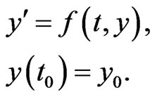 (B.1)
(B.1)
Initially, initial step size h is selected. Then the following algorithmic solution is used (Babolian, 1994), (Equation B.2) [9].
 (B.2)
(B.2)
The following equation is applied to obtain the values in the next iteration;
 (B.3)
(B.3)
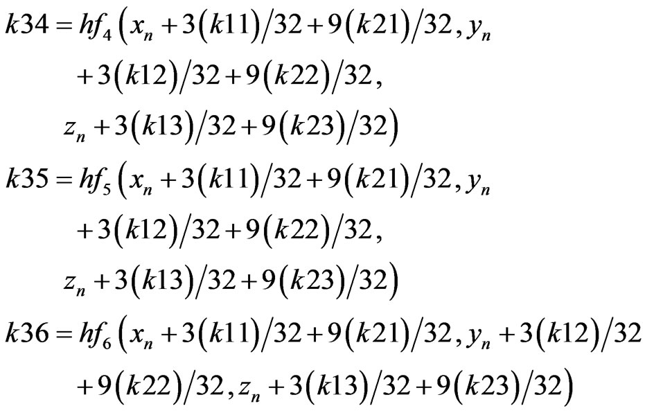
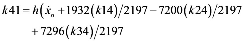
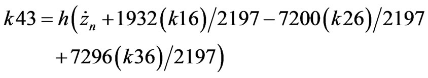
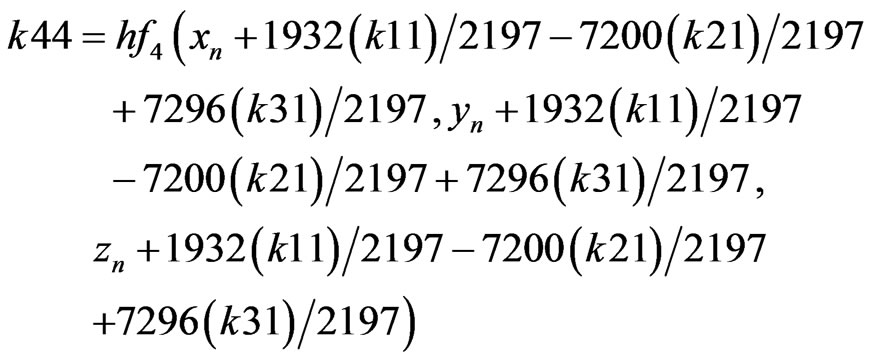
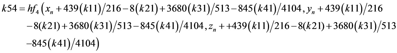
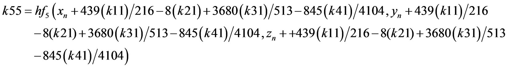
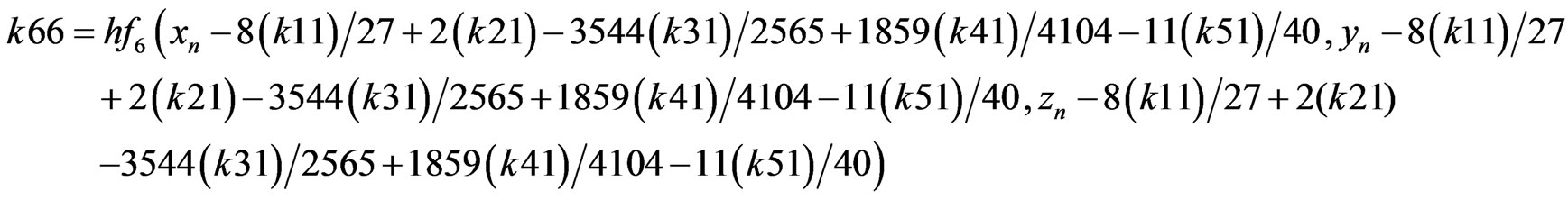
RKF coefficients are described as presented below (B.4) [8].
 (B.4)
(B.4)