Journal of Geographic Information System
Vol.5 No.2(2013), Article ID:29773,8 pages DOI:10.4236/jgis.2013.52011
LiDAR-Derived DEM and Raw Height Comparisons along Profile Corridor Gradients within a Forest
Forest Engineering, Resources, and Management Department, Oregon State University, Corvallis, USA
Email: Michael.Wing@oregonstate.edu, Michael.Craven@oregonstate.edu, John.Sessions@oregonstate.edu, Jeff.Wimer@oregonstate.edu
Copyright © 2013 Michael G. Wing et al. This is an open access article distributed under the Creative Commons Attribution License, which permits unrestricted use, distribution, and reproduction in any medium, provided the original work is properly cited.
Received November 12, 2012; revised December 15, 2012; accepted January 5, 2013
Keywords: LiDAR; Elevation; Profiles
ABSTRACT
We compared field based and airborne LiDAR-derived profile corridor measurements across forest canopy types and terrain ranging from 37% to 49% slope. Both LiDAR-derived DEM and raw LiDAR point elevations were compared to field data. Primary objectives included examining whether canopy type or terrain slope influenced LiDAR-derived profile measurements. A secondary objective included comparing cable logging payloads based on field measured profile elevations to payloads based on LiDAR-derived elevations. Average RMSE elevation errors were slightly lower for profile point to LiDAR DEM values (0.43 m) than profile point to nearest LiDAR elevation point (0.49 m) with differences being larger when sites within forest clearings were removed from analysis. No statistically significant relationship existed between field measured ground slopes and associated profile point and LiDAR DEM elevation differences but a mild correlation existed when LiDAR raw point elevation differences were compared. Our payload analysis determined the limiting payload distance and had consistent results across study sites. The DEM-based profile outperformed the nearest point profile by 5% on average. Results suggest that forest analysts should consider using the nearest LiDAR DEM value rather than the nearest LiDAR point elevation for terrain heights at discrete locations, particularly when forest canopy occludes locations of interest.
1. Introduction
Profile corridors are linear transects or pathways along which terrain gradients and elevations are measured. Measurements involve collecting elevation measurements at discrete points along a linear transect. Profile corridor measurements are typically collected to support cable logging operations but might also be gathered for various design projects including road and trail construction, fish passage creation, and stream channel restoration. Some applications, such as low volume road or recreational trail design may place a relatively low priority on accurate profile measurements. Other applications, such as reliable culvert placement or ensuring a level building structure footprint, may have greater requirements for accuracy.
Elevation measurements across a landscape can be collected using several different approaches. In support of these approaches, a variety of field and remote sensing measurement tools are available for profile corridor measurements. Profile corridor measurement techniques vary in cost, efficiency, and accuracy. Elevation data can be collected directly either through the use of differential leveling equipment or through global positioning system (GPS) receivers. Elevation can also be measured indirectly using analog vertical angle measurement equipment, such as an abney or clinometers, and tape measures to record distances between points. Trigonometry is then applied to calculate elevations. Electronic Distance Measurement (EDM) tools can also be applied to capture inclinations and distances for trigonometric elevation determination. A relatively new technology for collecting elevation measurements involves Light Detection and Ranging (LiDAR) sensors that are mounted on aerial platforms.
LiDAR sensors emit pulses of energy that come into contact with objects and then are reflected back toward the sensor. Pulse emissions are linked with an on-board GPS receiver and inertial navigation unit that associates a longitude and latitude coordinate with each returned pulse. The time that elapses when a pulse is emitted and its return to the LiDAR sensor is used to calculate the distance, referred to as a range, that the pulse traveled before striking an object. This range is used to associate an elevation value with the longitude and latitude coordinates ([1] Evans et al., 2009). LiDAR sensors can emit hundreds of thousands of pulses per second. Most LiDAR sensors are capable of capturing up to four separate returns for each pulse that is emitted. As pulses strike objects, a portion of the pulse is returned while other pulse portions may contain to travel. A first return is usually the first object struck by a pulse and is often associated with a taller landscape object, such as a tree or structure while last returns represent the ground surface or lowest point reached.
LiDAR elevation accuracies as stated by vendor specifications are typically around 0.15 m root mean squared error (RMSE). This level of accuracy, however, is generally only achievable under ideal conditions such as those encountered in flat, open terrain with minimal cover impediments for LiDAR pulses ([2] Reutebuch et al., 2003; [3] Hodgson and Bresnahan, 2004; [4] Su and Bork, 2006). Several previous studies have examined LiDAR elevation errors using a variety of approaches. While previous studies have considered the influence of slope gradient on LiDAR accuracy, the findings have not been consistent across studies and have involved relatively modest slope gradients.
[5] Kraus and Pfeifer (1998) found that LiDAR-derived digital elevation models (DEMs) were approximately as accurate as those created from photogrammetric techniques. Mean square errors for LiDAR DEMs were reported to be 0.57 m, with flat terrain accuracies being improved (0.25 m). [6] Gomes-Pereira and Janssen (1999) considered LiDAR DEMs for road planning applications and reported an RMSE range of 0.08 - 0.15 m on flat terrain, 0.25 - 0.38 m accuracy on sloped ground, and an overall RMSE of 0.29 m.
[2] Reutebuch et al. (2003) developed 347 elevation test points located in four forest settings including clearcut, heavily thinned, lightly thinned, and uncut using total station and GPS control measurements. Elevations from 1.5 m resolution DEMs were compared to the test points. Average elevation differences between test points and the LiDAR DEM were 0.22 m (0.24 SD) with a range from −0.63 m to 1.31 m. Average elevation differences were lowest for the clearcut site (0.16 m, 0.23 SD), moderate for the heavy (0.18 m, 0.14 SD) and lightly (0.18 m, 0.18 SD) thinned sites, and largest for the uncut forest sites (0.31 m, 0.29 SD). [2] Reutebuch et al. (2003) also examined the influence of LiDAR-derived slopes on LiDAR DEM accuracy and determined no influence but acknowledged some smoothing of elevations was likely present in their analysis.
[4] Hodgson and Bresnahan (2004) examined a 2 m resolution DEM and made comparisons to elevations determined by high order vertical control points across six land cover categories. RMSE values were greatest for deciduous forests (0.26 m) and lowest (0.17 to 0.26 m) for pavement, low grass, and evergreen forests. Elevation errors on steeper slopes (47%, 25˚) were estimated to be twice that found on lower slopes (3%, 1.5˚). [7] Hodgson et al. (2005) conducted a similar study within six land cover categories and reported a range of RMSE values from 0.15 to 0.36 m. The largest average error (0.36 m) occurred in scrub/shrub land cover. Reported RMSEs in pine, leaf-off deciduous, and mixed forests were 0.28, 0.27, and 0.24 m, respectively. Only the low grass land cover category exhibited increasing slope errors as terrain slope increased.
[4] Su and Bork (2006) examined the elevation accuracy of LiDAR-derived DEMs across 256 reference plots with elevations established by total station measurements. Treatment effects included slope, LiDAR sensor angle, and vegetation type (upland grassland, deciduous forest, shrub land, and riparian meadow). Several DEM interpolation methods were also evaluated (kriging, splining, and inverse distance weighting (IDW)). The reported overall project average elevation error and RMSE were +0.02 m and 0.59 m, respectively. Elevations tended to be underestimated in meadows but overestimated in forests. Both absolute elevation errors and RMSEs were found to increase as slope gradient increased.
We collected profile corridor measurements using rigorous field based techniques across a forested landscape that had also been measured using airborne LiDAR scanning. We compared field based and LiDAR derived profile corridor measurements across a range of different forest canopy types and terrain. Our primary objectives were to examine whether varying canopy cover and ground slope influenced LiDAR-derived profile corridor measurements. We examined both LiDAR-derived DEM and raw point elevations in our comparisons. Previous studies have typically only considered LiDAR-derived DEMs for LiDAR elevation accuracy assessments. A secondary objective included investigating a cable logging payload analysis based on field measured profile elevations and whether differences would result in the analysis if LiDAR-derived elevations were applied.
2. Methods and Materials
We included six sites in McDonald Research Forest (western Oregon, USA) for our study (Figure 1). Each site needed to contain enough area for four profile corridors. Other initial criteria for site selection included that both forested sites and a measurement control site free of overhead canopy during the LiDAR flight be included. Criteria for forested site selection included a range of
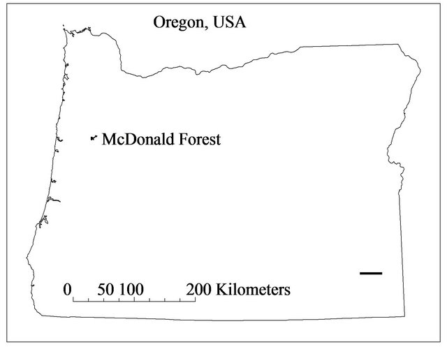
Figure 1. Location of McDonald Forest in Oregon, USA.
stand characteristics representing trees per ha, basal area, and conifer/hardwood forest be represented across the sites, and that sites should not include any standing timber that had been harvested in a 20 years period previous to the LiDAR flight (Table 1). We also strove to find areas that had been thinned or harvested since the LiDAR flight in order to improve field data collection operations.
In terms of a measurement control site, we initially included a clearcut area but became concerned upon visiting the site that on-the-ground harvesting residue present during the LiDAR flight might bias ground elevations from the LiDAR. We retained the clearcut site but also chose to include an open meadow site as measurement control. At all forest sites, including the clearcut site, another criterion was that ground slopes exceed 35% on average. This slope threshold is often associated with forested areas that require cable logging. We relaxed this slope requirement for the meadow site as no other open areas were available in the research forest that met all other criteria.
We measured elevation at points located along four profile lines at each study site. Points were taken along each profile at changes in the ground slope. If there was no appreciable change in ground slope, we attempted to maintain a maximum spacing between points of approximately 7.5 m. Average point spacing was below 7.5 meters, but due to field conditions some profiles had average spacing greater than 7.5 meters.
Study site corridor points were measured using one of two field surveying techniques. Selection of field surveying technique varied depending on whether each site had canopy or notduring field measurements. The meadow, clearcut, low forest density, and mixed forest sites were either already free of canopy or had been clearcut following the LiDAR flight. These four sites were surveyed with Real Time Kinematic (RTK) GPS using a survey-grade GPS receiver. A measurement control point was set at each site and a static four hour or longer GPS observation was conducted. GPS observations were then processed into a control point using the National Geodetic Survey’s Online Positioning User Service (OPUS). Using the control point as the base station for the RTK surveying, elevation points were measured along the profile corridors at each of the four sites. We used preset stakeout points to control the profile azimuth during RTK GPS surveying.
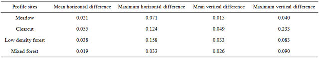
Extra points were taken along each profile to provide some measure of the precision of the RTK measured points. Every fifth point that was measured during the initial pass along the profile was staked and marked. After a period of at least 15 minutes, which allowed the satellite constellation to move, the staked points were revisited and measured a second time. The difference in horizontal distance and elevation values were calculated for each pair of repeated points. Average vertical height differences were 0.055 m or less for all sites (Table 2).
The medium and high forest density sites each had canopy conditions that made GPS surveying impractical. Profile points at each of these sites were measured with a digital total station. Measurement control was created at each site by using the nearest canopy opening that would support an unobstructed GPS observation. Two control points are required when using a total station: one point is used to establish control coordinates while the second point establishes the orientation of the total station. Initial control coordinates were provided by a minimum four hour static GPS observation that was processed with OPUS. The second point was set using a three minute RTK observation based on the OPUS control point to establish the angular orientation. For both sites, two total station setups were required to get from the control location to the designated profile site.
Once measurement control had been established at the medium and high forest density sites, total station measurements were collected along the corridors. To reduce potential errors in the digital total station measurements, repeat backsights were taken during all instrument setups. After each backsight and subsequent measurements for an instrument setup were completed, the backsight point was re-measured. The original backsight point and the re-measured point were inversed during the course of the survey to ensure that a blunder had not been made. Profile corridors were kept in alignment by locking the azimuth of the total stations during all measurements.
The LiDAR data used in this study were flown by Watershed Sciences, Inc. of Corvallis, Oregon. The data were collected in April 2008, which was still in the “leaf-off” period for that year. The laser scanner used was a Leica ALS 50, which is capable of recording four returns per laser pulse, and produces a native density of eight plus points per square meter. Total LiDAR returns averaged 10 points/m2 across the forest and ground re-
Table 1. Profile site characteristics.

Table 2. Re-measured Real Time Kinematic GPS elevation differences (m).
turns averaged 1.12 points/m2 ([8] Watershed Sciences 2008). Raw point returns were provided as well as a one meter resolution DEM. The LiDAR data were registered to Universal Transverse Mercator (UTM) coordinates using the NAD 83 (CORS96) datum. The OPUS solutions on the control points were also available in the same UTM coordinates and datum, so both field and LiDAR data were in the same spatial map projection.
Our analysis involved two initial comparisons between field measured profile point elevations and LiDARderived elevations. First, for each profile point elevation that was surveyed in the field, we subtracted the LiDAR DEM value that was associated with the same location. Second, we also subtracted the nearest LiDAR point elevation from each profile point elevation. These calculations were performed with a geographic information system (GIS). We also investigated whether ground slopes influenced differences between field measured and LiDAR-derived elevations. The ground slope associated with each profile point was calculated by taking the average of the percent slope as indicated by field measurements to the next uphill and next downhill points. In the case of the initial profile point, we only used the next downhill point slope; for the final corridor point, only the next uphill point slope was used.
We relied upon root mean square errors and average errors between the field surveyed and LiDAR elevations for descriptive statistical comparisons. For statistical analysis, we used the absolute value of elevation differences in order to avoid compensating errors from using average differences. Statistical testing procedures included analysis of variance (ANOVA) and Tukey multiple range tests. We used a base 10 logarithmic transformation of the absolute errors so that data distributions approximated normality and supported parametric statistics.
We also conducted a third comparison that considered a cable logging payload analysis based on field measured profile elevations and differences that resulted by using LiDAR-derived elevations for the same profiles. The primary reason for creating profile corridors is to determine the limiting payload for a cable logging operation (Figure 2). Our third comparison considered the differences among payloads associated with the three data sources. The steepest profile was selected from each of the six sites for payload analysis. Three versions of the each profile were analyzed and included field measured elevations, LiDAR DEM elevations, and nearest LiDAR point elevations. The analysis software was Skyline XL which enables payload analysis within an Excel spreadsheet interface. Skyline XL is produced by the US Forest Service and is freely available ([9] USFS, 2010).
Each profile was analyzed using the same parameters so that relative comparisons could be made with one exception. Key parameters included cable system, yarder and carriage combination, rigging heights, log sizes, and clearances (Table 3). While most profiles allowed a 9.1 m tailspar, the medium and high density forest profiles both required a tailspar 15.2 m eliminate feet above ground to support a payload. Under actual conditions, one might
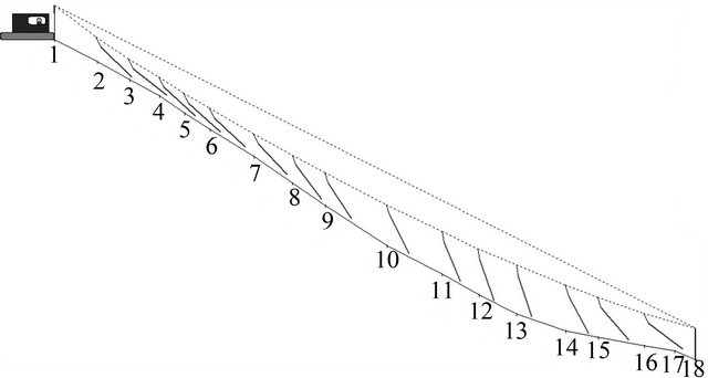
Figure 2. Clearcut profile No. 1 skyline system.
Table 3. Profile analysis parameters.
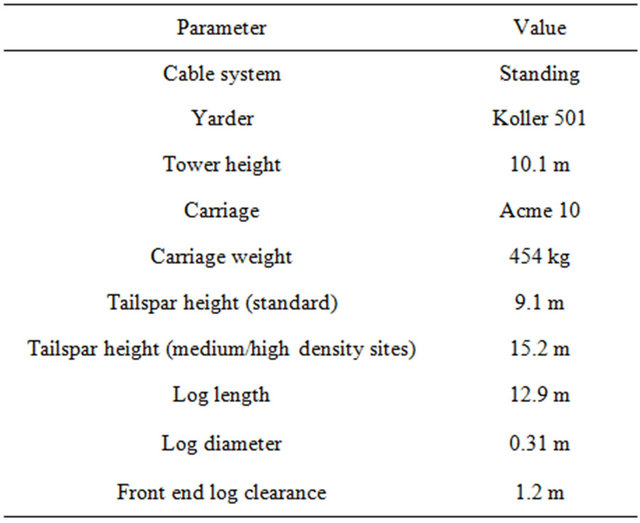
consider a multi-span setup rather than a taller tailspar with a single span skyline but our common parameter set enables comparisons between the three elevation sources nonetheless. We used a relatively smaller tower (10.1 m) for our payload analysis. The choice of a smaller tower over a larger tower likely accentuates the differences in payload capacity between the three elevation sources.
3. Results
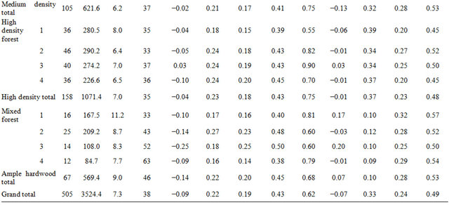
We measured the elevations of 505 profile points covering 3524 m of profile corridors at the six study sites (Table 4). The smallest number of profile points was collected at the low forest density site (39) while the largest number was collected at the high density forest site (158). Overall, there was an average of 7.33 m that separated profile point locations within the corridors. The lowest average point separation occurred in the medium density forest site (6.15 m) while the highest was in the mixed forest site (9.04 m).
3.1. Profile Point and DEM Elevations
We subtracted LiDAR DEM values from the profile point elevations to determine RMSE, average, and standard deviation (SD) of elevation differences (Table 4). The meadow site had the lowest overall average elevation RMSE (0.38 m) and the clearcut site had the highest (0.50 m). The four forested sites had average RMSE values that ranged from 0.41 to 0.46 m. The overall average elevation differences for DEM values were negative for all study sites with a combined average of −0.09 m (SD 0.22). This indicates that LiDAR DEMs tend to overestimate actual heights. We found that there were statistically significant differences between the profile point and DEM elevation differences among the six study sites (p = 0.03). The medium forest density site had the lowest average elevation error (−0.02 m, 0.21 SD) and the clearcut site had the highest (−0.22 m, 0.19 SD). A Tukey multiple range test determined that these were the only two study sites that were statistically different from one another. Two other study sites, however, had individual corridors with positive elevation differences. This included corridors 3 (0.03 m) and 4 (0.02 m) on the medium density forest site and corridor 3 on the high density forest site (0.03 m).
We also tested whether field measured ground slopes were related to profile point and DEM elevation differences, and found no statistically significant association (p = 0.21).
3.2. Profile Point and Nearest LiDAR Point Elevations
We compared the elevation of each profile point to the nearest LiDAR point by subtracting LiDAR point elevations. Overall, the nearest LiDAR point was located an average of 0.62 m from the nearest profile point (Table 4). Average distances were smallest for the meadow (0.32 m) and clearcut (0.33 m) sites. Average separation distance was relatively consistent for the forested sites and ranged from 0.68 m for the mixed forest site to 0.75 m for the medium and high density forested sites. We used regression to test the influence of profile point and nearest LiDAR point separation difference and found no statistically significant differences (p = 0.98).
Average elevation RMSE for nearest LiDAR point was 0.49 m across all study sites. Nearest LiDAR elevation comparisons were lowest for the meadow site (0.35 m) and highest for the low density forest site (0.57 m). The other three forest categories had RMSEs that ranged between 0.48 m (high density forest) and 0.53 m (medium density forest and mixed forest). The clearcut site had a RMSE of 0.49 m.
Average elevation differences for the nearest LiDAR point were −0.07 m across all six study sites but included considerable variation (0.33 SD) and two sites with average differences that were not negative (low density forest (0.01 m) and mixed forest (0.07 m)). Among the 24 individual corridors, there were six corridors at three sites that had positive average elevation differences. The overall trend, however, suggests that LiDAR elevations
Table 4. Profile measurement results (units in m).

over estimate actual heights.
We found statistically significant differences in the average elevation differences between profile point and LiDAR point elevations (p < 0.01). Tukey multiple range tests determined that the meadow site was different from the clearcut, medium density, and mixed forest sites. The lowest average elevation difference was determined at the low density forest (0.01 m) and high density forest (−0.01 m) sites. The maximum elevation average elevation difference was measured at the clearcut site (−0.23 m).
Field measured ground slopes were determined to be related to average elevation differences between profile point and LiDAR point elevations (p < 0.01) but the correlation was not strong (r2 = 0.01).
3.2. Payload Analysis
For each profile the critical terrain point or the point that caused the limiting payload occurred at the same distance from the yarder regardless of the elevation source (field measured, DEM-derived, and nearest raw LiDAR elevation). We anticipated this result as elevation difference between the three elevation sources were relatively small, resulting in the same general geometry for each profile.
Using the field measured profiles as a base line, the percent difference in limiting payload was calculated for the DEM elevation and nearest point elevation profiles. On average, the DEM based profiles underestimated the limiting payload by 6%, with a range of 39% below to 18% over estimation. The nearest point based profiles performed worse with an average overestimation of 11% and a range of 20% below to 39% above.
4. Discussion
We found that average RMSE elevation errors were slightly lower for profile point to LiDAR DEM values (0.43 m) as contrasted to profile point to nearest LiDAR elevation point (0.49 m) comparisons across our six study sites. The elevation differences between these two methods of extracting elevations from LiDAR are relatively small and likely have little influence on applications such as terrain and hydrologic modeling but may influence engineering efforts that involve design applications. The elevation differences become more pronounced however when the four forested sites are considered and the meadow and clearcut sites are not. Average RMSE values for the four forested sites were 0.43 m for the LiDAR DEM and 0.53 m for the nearest LiDAR point.
One possible explanation for the lower LiDAR DEM errors when contrasted to nearest LiDAR point elevation errors could be the distance that separated field-collected profile points from the nearest LiDAR elevation. The average separation distance was 0.62 m but some differences in individual corridors reached nearly a meter. LiDAR DEMs represent an interpolated surface that is based on an averaged elevation created from a neighborhood of raw LiDAR points. The interpolated surface may represent a better fit that the nearest point due to the terrain elevation averaging, particularly as nearest distances increase.
Our overall RMSE results for LiDAR DEM values (0.43 m) as contrasted to profile point to nearest LiDAR elevation point (0.49 m) are lower than those reported by one previous study that focused on DEM elevation comparisons ([4] Su and Bork, 2006). However, our errors were higher than those reported by several earlier studies that utilized LiDAR-derived DEM elevations ([6] Gomes-Pereira and Janssen, 1999; [3] Hodgson and Bresnahan, 2004; [7] Hodgson et al., 2005). There are doubtlessly site factors that influence the differences. For instance, our average slope gradients (38%) exceeded those reported by several of the studies ([3] Hodgson and Bresnahan, 2004; [7] Hodgson et al., 2005; [4] Su and Bork, 2006). We note that while [3] Hodgson and Bresnahan, 2004, considered 47% slopes, results were based on scaling the results from lower slope values. It is also unlikely that forested sites were very similar in structure between any two studies. In addition, seasonality and LiDAR technology (hardware and software) also influence study results.
RMSE values have been typically used by previous LiDAR elevation studies but at times average errors have been the focal statistic. Our overall average errors for LiDAR DEM values (−0.09 m) and nearest LiDAR elevation point (−0.07 m) were lower than the overall average (0.22 m) reported by a previous study ([2] Reutebuch et al. 2003). The site slopes in our study, however, were greater than those reported by [2] Reutebuch et al. 2003. Given the advances in scanner technology that have occurred since this earlier study, we would anticipate reduced errors. In addition, the density of LiDAR pulses was enhanced in our study (10 points per m2) in comparison to the earlier study (4 points per m2).
Some previous studies determined an association between steeper slopes and increased errors in LiDAR elevations ([5] Kraus and Pfeifer, 1998, [6] Gomes-Pereira and Janssen, 1999; [3] Hodgson and Bresnahan, 2004, [4] Su and Bork, 2006) while other studies have either not found a correlation ([2] Reutebuch et al., 2003) or determined an inconsistent relationship depending on study site. [7] Hodgson et al. (2005) found that only the low grass land cover category exhibited increasing slope errors as terrain slope increased.
We found no statistically significant association of field measured ground slopes to profile point and DEM elevation differences (p = 0.21). We did, however, discover that field measured ground slopes were significantly related to average elevation differences between profile point and LiDAR point elevations (p < 0.01) but the correlation was relatively weak (r2 = 0.01). Given these results, it appears that greater slopes may have at times a small influence on LiDAR accuracies but the influence is likely negligible within the study sites in our study. This finding may be a result of the way in which we determined ground slopes at our field sites. Ground slopes were determined based on the average slope between each profile point and its upslope and down slope neighboring profile points.
Payload analysis is at times an inexact process, as a large number of variables can affect results. We held most of the variables in our analysis constant with the exception of the tailspar height. Our payload analysis considered where the limiting payload occurred relative to the yarder and results were consistent among all study sites. The DEM-based profile appeared to outperform the nearest point profile by 5% on average and appears to be the preferred LiDAR elevation source for payload analysis.
Our results suggest that forest analysts should consider using the nearest LiDAR DEM value rather than the nearest LiDAR point elevation for terrain heights at discrete locations, particularly when forest canopy occludes locations of interest. We base this recommendation on the slightly improved performance of the LiDAR DEM over the nearest LiDAR point profile elevation comparisons, and note that further performance increases when only forested sites were concerned.We also observed an improved performance of the LiDAR DEM in our payload analysis.
In addition, with DEMs being readily accessed in GIS packages it is typically easier for an analyst to access and manipulate a LiDAR DEM-derived profile rather than trying to draw values from the nearest point elevations. This circumstance lends more incentive to use LiDAR DEMs as a source of elevation data.
5. Conclusions
Our primary investigation was to determine whether canopy type or terrain slope influenced LiDAR-derived profile measurements. We also compared cable logging payloads based on field measured profile elevations to payloads that were based on LiDAR-derived elevations. To support these investigations, we compared field based and airborne LiDAR-derived profile corridor measurements in different canopy types and on moderate slopes. Our field based measurements were compared to both LiDAR-derived DEM and raw LiDAR point elevations The profile point to LiDAR DEM RSME values we determined was slightly lower (0.43 m) than the profile point to nearest LiDAR elevation point RSME (0.49 m). These differences became enhanced when study sites that occurred in forested clearings were not included the analysis. We found no statistically significant relationship between field measured ground slopes and associated profile point and LiDAR DEM elevation differences.
We determined the limiting payload distance and found consistency in our findings regardless of study site. The DEM-based profile resulted in 5% improvement on average. Our results encouraged forest analysts that use LiDAR data to support operations should work with the nearest LiDAR DEM value rather than the nearest LiDAR point elevation for terrain heights at discrete locations, particularly under forest canopy. LiDAR-based DEMs are often provided by LiDAR vendors, require less storage than LiDAR point elevations, and are generally easier to work with.
REFERENCES
- J. S. Evans, A. T. Hudak, R. Faux and A. M. S. Smith, “Discrete Return LiDAR in Natural Resources: Recommendations for Project Planning, Data Processing, and Deliverables,” Remote Sensing, Vol. 1, No. 4, 2009, pp. 776-794. doi:10.3390/rs1040776
- S. E. Reutebuch, R. J. McGaughey, H.-E. Andersen and W. W. Carson, “Accuracy of a High-Resolution LiDAR Terrain Model under a Conifer Forest Canopy,” Canadian Journal of Remote Sensing, Vol. 29, No. 5, 2003, pp. 527-535. doi:10.5589/m03-022
- M. E. Hodgson and P. Bresnahan, “Accuracy of Airborne LiDAR-Derived Elevation: Empirical Assessment and Error Budget,” Photogrammetric Engineering and Remote Sensing, Vol. 70, No. 3, 2004, pp. 331-339.
- J. Su and E. Bork, “Influence of Vegetation, Slope, and LiDAR Sampling Angle on DEM Accuracy,” Photogrammetric Engineering and Remote Sensing, Vol. 72, No. 11, 2006, pp. 1265-1274.
- K. Kraus and N. Pfeifer, “Determination of Terrain Models in Wooded Areas with Airborne Laser Scanner Data,” ISPRS Journal of Photogrammetry and Remote Sensing, Vol. 53, No. 4, 1998, pp. 193-203. doi:10.1016/S0924-2716(98)00009-4
- L. M. Gomes and L. L. F. Pereira, “Janssen Suitability of Laser Data for DTM Generation: A Case Study in the Context of Road Planning and Design,” ISPRS Journal of Photogrammetry and Remote Sensing, Vol. 54, No. 4, 1999, pp. 244-253. doi:10.1016/S0924-2716(99)00018-0
- M. E. Hodgson, J. Jenson, G. Raber, J. Tullis, B. A. Davis, G. Thompson and K. Schuckman, “An evaluation of LiDAR-Derived Elevation and Terrain Slope in Leaf-Off Condition,” Photogrammetric Engineering and Remote Sensing, Vol. 71, No. 7, 2005, pp. 817-823.
- Watershed Sciences, “LiDAR Remote Sensing Data Collection: McDonald-Dunn Research Forest,” Watershed Sciences Inc., Corvallis, 2008.
- United States Forest Service (USFS), “Index of Programs,” 2010. http://www.fs.fed.us/r6/nr/fp/FPWebPage/FP70104A/Programs.htm