Journal of Geographic Information System
Vol. 4 No. 3 (2012) , Article ID: 19592 , 15 pages DOI:10.4236/jgis.2012.43024
Detection of Land-Use and Surface Temperature Change at Different Resolutions
Soil and Water Department, Faculty of Agriculture, Suez Canal University, Ismailia, Egypt
Email: ee.omran@gmail.com
Received February 27, 2012; revised March 15, 2012; accepted April 1, 2012
Keywords: Remote Sensing; GIS; Landsat Image; Land-Use; Change Detection; Surface Temperature; Ismailia
ABSTRACT
Understanding the relationship between land-use/land-cover change (LULCC) and environment is seriously important to manage arid land. However, information on how environmental factors influence the LULCC patterns at different scales in arid area is lacking. This paper investigates the application of RS/GIS for detecting LULCC and assessing its impact on surface temperature in the Ismailia Governorate, Egypt. Landsat images have been utilized to quantify the changes from 1984 to 2011. The images were pre-processed using calibration techniques and the geometric and atmospheric corrections were performed. Different ratios, indices, and optimized index factor were implemented to decide the best band combination. Supervised classification using Maximum Likelihood technique and spatial reclassification have been employed. Six land-use/land-cover categories (urban, vegetation, waterlogged 1 and 2, bare land, and water) were identified. The highest overall accuracy and Kappa coefficient is 93.04% and 80.65%, respectively. The integration of RS and GIS was further applied to examine the impact of land-use change on surface temperatures. The results revealed a notable land-use change in the study area. The Built-up area has rapidly increased in Ismailia during the 27 years period. The built-up area (37.65˚C in 1984 and 43.876˚C in 2011) and Barren land (37.34˚C in 1984 and 42.801˚C in 2011) exhibit the highest surface radiant temperature, while vegetated surfaces (28.73˚C in 1984 and 32.96˚C in 2011), water (25.94˚C in 1984 and 27.32˚C in 2011), waterlogged 1 (34.54˚C in 1984 and 35.60˚C in 2011) recorded low radiant temperature respectively. Waterlogged 2 is the class that shows an unexpected radiant temperature (26.38˚C in 1984 and 27.75˚C in 2011). The urban development between 1984 and 2011 has given rise to an average of 6.23˚C in surface radiant temperature. During 27 years, the change rate of land-use types which are decreased are barren land (1.12% annually) and waterlogged 1 and 2 (0.76 and 6.61% annually). The area of vegetation, water, and built-up are increased by 0.98%, 0.82%, and 0.61% per year, respectively.
1. Introduction
The wide range of spatial, spectral and temporal scales is one of the most important and difficult aspects of soil science [1,2]. It covers spatial scales from the molecular to the landscape, and temporal scales from instantaneous processes to soil formation processes. Some discrepancies are presented between the spatial scale at which a process is modeled (e.g. “up-scaling” or “down-scaling”), and the scale at which a policy maker needs to make decisions (field, farm, regional or national scale). Land-use change has been considered a local environmental issue, but it is also has environmental implications at regional levels, and are becoming central issues in the study of global environmental change [3-7]. Dealing with scaling issues will be central to progress in land-use and landcover change (LULCC). Unplanned changes of land-use are a major problem. Most land-use changes occur without a clear and logical planning with any attention to their environmental impacts. The problems of haphazard, air pollution, urban growth, soil erosion, desertification, and loss of prime agricultural lands cannot be well understood and mitigated without the knowledge of LULCC at different scales that drives them. These problems pose the question “Is scale matters?”
At the spatial scale, Omran (2009) develops a methodology to improve land-use mapping accuracy for the Ismailia Governorate, Egypt [8]. However, is the accuracy of this method worth being worked for its change detection at temporal scale? Change detection in land-use and land-cover can be performed also on a temporal scale such as a decade to assess landscape change caused due to anthropogenic activities on the land [9-12]. Land-use and land-cover are dynamic in nature and are important factors for the interaction and relationship of anthropogenic activities with the environment. However, because satellites observe land-cover, but not land-use, the effort to link remotely sensed observations of the landscape with human activity on the ground requires data different from conventional remote sensing studies. Land-use change is more difficult to map than land-cover change because the former requires an understanding of the anthropogenic use of the land and not simply land-cover characteristics. The first goal of this paper is “to spatially and temporarily map land-use change patterns in the Ismailia over the period of time 27 years”.
At the spectral scale, the mapping land-use changes are the first step in evaluating the impact of aggressive agricultural practices on the surface temperatures in the arid environment, such as Ismailia Governorate. Agriculture is difficult to characterize because of the spectral complexity of crop phenology and the variety of agriculture forms. Knowledge of land surface temperatures is necessary for a wide range of environmental studies and applications. Land surface temperatures are most important in global change studies as they are use in the estimation of radiation budget, heat balance and in climatic modeling [13]. Studies of surface temperature have been conducted primarily using NOAA AVHRR data [14-17]. The 1.1 km resolution of these data is found suitable only for small-scale temperature mapping. [18-20] have used the TM thermal infrared data to observe mesoscale temperature differences between urban, and rural areas. According to my knowledge, no research has yet attempted to detect surface temperature change over time at a local level using multi-date ETM+ thermal infrared data. So, the second goal of this paper is “to analyze the impact of LULCC on the land surface temperature (spectrally) in Ismailia Governorate at a local level”.
Change detection method is useful in different applications such as LULCC analysis, monitoring of shifting cultivation, study of changes in vegetation phenology, seasonal changes in crop production, crop stress detection, disaster monitoring, and other environmental changes. Knowledge of the present land-use, agricultural area, as well as information on their changing proportions, is needed by legislators, planners, and local governmental officials to determine better land-use and land evaluation policy. The results may support policy-makers to achieve long-term sustainability of land and water resources and its impacts on climate change.
2. Study Area
Ismailia Governorate, Egypt was selected to be the investtigated site for the study undertaken. It is located in northern part of Egypt between 31˚40' to 32˚50' Longitude and 30˚10' to 31˚00' Latitude, (Figure 1). The choice of the Ismailia Governorate implies that the local specific land-cover/land-use is represented. The climate of Ismailia Governorate is of arid type that is experiencing significant land-use change due to an extensive irrigation system that is converting semi-natural areas into arable land.
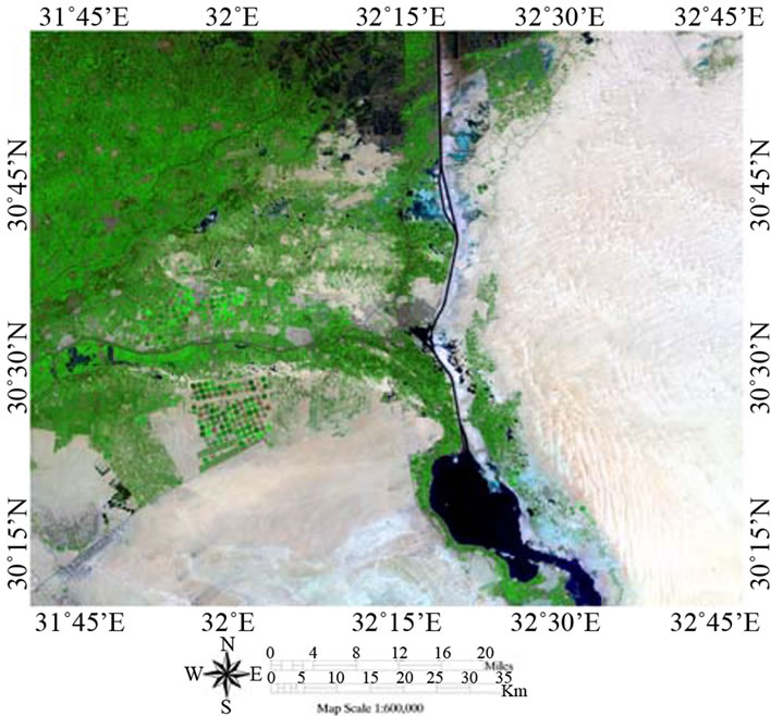
Figure 1. Satellite image for the study area.
Environmental protection in Ismailia Governorate has been faced critical problems due to several factors as the increasing population, demolishing natural resources, environmental pollution, land-use planning as well as others. The Ismailia Governorate covers an area of 539426.43 Hectare [21].
3. Methodology
The overall research methodology steps are reveled in Figure 2.
3.1. Data Acquisition and Preprocessing
A reconnaissance visiting was performed for the study area to get acquainted with different land-use and landcover patterns. The extensive field surveys were guided with a Global Positioning System (GPS) receiver. The data collected during the field surveys were used for four major purposes. The first is to determine the major types of land-use in the study area, which helped design a land-use and land-cover classification procedure. The second is to associate the ground “truth” of a specific type of land-use with its imaging characteristics, which helped classify images and produce land-use maps. The third is helped to determine the anthropogenic activities of landuse. Finally is to collect sufficient data for image preprocessing. In addition, visual analyses of the enhanced images were carried out with the assistance of field and ancillary data such as knowledge-based, existing land-use, and topographic maps.
Land-use patterns for 1984, 2006 and 2011 were mapped by the use of Landsat images (Dates: 20/09/1984, 04/12/2006 and 10/04/2011). Acquisition of different high quality dated imagery is available from numerous public and private sources. The Landsat ETM+ imagery
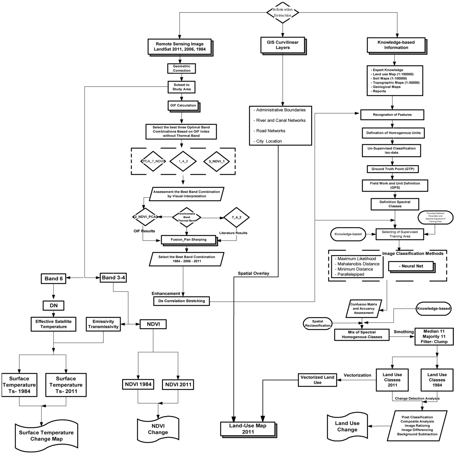
Figure 2. Flow chart for the research methodology on land-use change detection.
of 2006 and 2011 was subject to “data gaps” owing to the failure of Scan Line Corrector (SLC) of ETM+ instrument in 2003. Therefore, “Data Masking” was performed after stacking each band of 2006 and 2011 images together.
The data gaps in the imagery correspond to a DN value of “0” and hence they were masked out prior to processing, the rest of the data corresponds to a DN value of 1. To determine the best band set, OIF and correlation method were used [8]. All the bands (1-6 without thermal band) plus Normalized Difference Vegetation Index (NDVI) and Principal Component Analysis (PCA) were used to calculate OIF. The role of high OIF values is to give more spectral information of the object.
The band combination with the highest OIF has the highest variance and lowest duplication for the scene, and thus contains the greatest amount of information about the scene (Figure 3). The Environment for Visualizing Images (ENVI 4.8) was used to process and analyze the data.
According to Figure 3, the highest OIF (54.22) for 2011 image is allied to band set: 4, 1 and 3. Also the highest OIF (95053.19) for 2006 image is allied to band set: 2, NDVI and PCA. However, for 1984 image, the highest
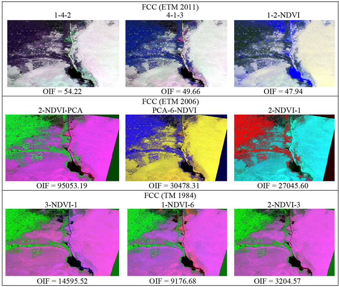
Figure 3. The highest OIF values for different spectral composite at different temporal and spectral scales. Key: FCC = False color composite, 1 - 5 = normal band, 6 = band 7, OIF = Optimum index factor, NDVI = Normalized difference vegetation index, PCA = Principal component analysis.
OIF (14595.52) is allied to band set: 3, NDVI and 1. Correlation among bands demonstrates that the bands 1-4-2 for 2011 image, 2-NDVI-PCA for 2006 image, and 3-NDVI-1 for 1984 image are a suitable set for land-use mapping. The classification accuracy is high when these bands are used instead of using all bands. It can be concluded that this is due to the high correlation among bands. High correlation among bands means replication of data according to Sabins (1996) [22].
3.2. Spectral Classification and Spatial Reclassification
ISODATA (Interactive Self-organizing Data Analysis) algorithm was applied as a preliminary step to identify and classify spectral clusters from image data excluding the thermal band. The aim of the image classification process is to convert image data to thematic data. The supervised classification was executed using the different classification algorithm, supported by visual interpretation and the application of post processing techniques. Training samples were first selected from various spectral classes. After selecting the training samples, classifycation was run on the data using different methods and algorithm. Grouping of spectral classes were done on the basis of land-cover types. Therefore, further research effort was attempted to reduce image classification errors and improve accuracy. For this purpose, a spatial reclassification procedure has been developed to recode those pixels being labeled wrongly.
Spatial reclassification was implemented through the use of image interpretation procedures, knowledge-based approaches, auxiliary data, and a variety of GIS functions. More than 100 digital photos were taken for different types of land-use and land-cover, along with hundred of GPS point readings.
3.3. Spatio-Temporal and Spectral Change Detection Techniques
There are numerous change detection techniques and analytical methods that can be employed to achieve LULCC. Spectral change detection methods are as follows [23]: Image differencing, image rationing, image regression, change vector analysis, vegetation index differencing, manual on-screen digitization of change, and multidate principal component analysis. Change detection approaches can be broadly divided into either post-classifycation or pre-classification (spectral) methods. Post-classification uses two or more images from different dates and classifies them independently. However, pre-classification or spectral techniques rely on the principle that LULC changes result in persistent changes in the spectral signature of the land surface. These techniques involve the transformation of two original images to a new single-band or multi-band image in which the areas of spectral change are highlighted. Classification techniques can take the form of unsupervised, supervised, or a combination of both techniques.
In the present study, post-classification method which determines the difference between independently classified images from each of the different dates is used. Later, the classification results are compared directly and the area of changes extracted [24-27]. It is the only method in which from and to classes can be calculated for each changed pixel. Supervised and unsupervised classifications are used in this approach. Individual classification of two image dates minimizes the problem of normalizeing for atmospheric and sensor differences between two dates [26]. A change matrix for LULCC between 1984 and 2011 were produced.
3.4. Impact Analysis of Land-Use Scale on Climate Change
All the three Landsat images have been geometrically rectified and geo-referenced to UTM Zone 36˚ North, WGS- 84 Datum. The Landsat images are available in uncalibrated format unsuitable for any spectral analysis, hence, calibration of images into units of spectral reflectance was performed by first converting uncalibrated Digital Number (DN) units to calibrated radiance by using the following linear equation [28]:
 (1)
(1)
Thereafter, the spectral radiance was converted into spectral reflectance through the following equation:
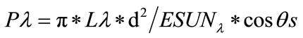 (2)
(2)
where, Pλ is the planetary spectral reflectance, Lλ is solar reflected radiance calculated in Equation (1). (d) is the Earth-Sun distance at the Julian date (Table 1) of the image in astronomical units (AU), ESUNλ is the incoming solar spectral irradiance in that waveband (W/m2/μm), θs is solar zenith angle in (˚).
This enables the pixels of the images in identification of their spectral properties.
In examining the spatial relationship between land-use types and the surface energy response as measured by Tsthe classified land-cover images in 1984 and 2011 were overlaid to the Ts image of corresponding years. Also, normalized difference vegetation index (NDVI) image was computed for 1984 and 2011 from visible (0.63 - 0.69 mm) and near-infrared (0.76 - 0.90 mm) data of the Landsat TM, and ETM+ using the following formula:
 (3)
(3)
NDVI has been found to be a good indicator of surface radiant temperature [29-34]. Surface temperature change image between 1984 and 2011 was also produced using image differencing. This image was overlaid with the land-use change map and with the NDVI change map to study how all these changes have been interacted.
3.5. Yearly Change Rate of a Land-Use Type
The land-use type change is the result of land conversion. It involves the conversion of one particular land-use type i to another type j and the conversion of land-use type i from type j. Although there are several models to describe the conversion trends among the land-use types [35,36], this study uses the real data obtained from the field survey of land-use types. The Transformation Rate (TRi) for each land-use type was calculated as [37]:
 (4)
(4)
where TRi is the transformation rate of land-use type i in a monitoring period from t1 to t2, and LA (i, t1) – ULAi represents the area of land-use type i converted to other types in the period with LA (i, t1) being the area of type i at the beginning of the period and ULAi being its unchanged area during the period. The Increasing Rate (TRi) of land-use type i is expressed as:
 (5)
(5)
where LA (i,t2) – ULAi represents the area of land-use type i converted from other land-use types, i.e., newly created land-use type i, in the monitoring period and LA (i,t2) is the area of land-use type i at the end of the monitoring period, and ULAi is the same as above. The Change Rate (CRi) of land-use type i is then:
 (6)
(6)
A positive CRi indicates the area of type i land-use was increasing, while negative indicates it was decreasing.
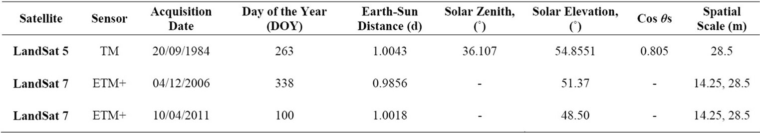
Table 1. The used Landsat data.
3.6. Accuracy Assessment and Map Presentation
Accuracy assessment is a guide to map quality and reliability [38]. The value of the final map is a function of the accuracy of the classification. The accuracy assessment was conducted through a standard method described by [39] and was calculated using an error matrix [40] which showed the accuracy of both the producer and the user.
The classification accuracy in remote sensing shows the correspondence between class labels allocated to pixel and true class. The true class can be observed in the field directly or indirectly from a reference map [41]. A random distribution of such sampling points over the whole region must be sought [42]. At least 20 test points per class were taken through a stratified random sampling scheme. For accuracy assessment, 250 pixels were randomly selected from the ground truth coverage. Land-use maps and photographs taken for documentary purposes were used as a reference data to observe true classes. The overall accuracy and a Kappa analysis were used to perform a classification accuracy assessment based on error matrix analysis. A standard for land-use maps is set between 85% [43-45] and 90% overall accuracy.
Raster data was preprocessed to reduce the large amount of data. Before conversion to vector format, the image was simplified to reduce the pixel by pixel classification to some smaller number of polygons. Raster to vector translation was occurred for the purpose of presentation and analysis in a GIS layer. The vector files of rivers, roads, and administrative boundaries for Ismailia were overlaid on the vector land-use map to update roads, rivers and boundary features through screen digitization in ESRI ArcMap v 10.0 [46].
4. Results and Discussion
4.1. Data Processing and Spectral Classification
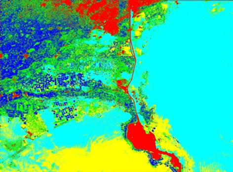
Figure 4 shows the results of ISODATA classification. The Landsat ETM+ image was first classified to 8 landuse types which are identified based on its spectral signature including: urban or built-up land, barren land, vegetation, reed vegetation, trees areas, water and waterlogged 1, 2 area.
After that, supervised classification was performed using the different classification algorithm. Table 2 shows the accuracy of different classification methods and algorithms. Neural network and maximum likelihood methods have a good result on out coming maps.
The overall accuracy and Kappa coefficient of these methods are quite higher than the other algorithms such as: Minimum distance and parallelepiped classifiers. [47, 48] have emphasized the priority of maximum likelihood algorithm in comparison to minimum distance and parallelepiped classifiers. Overall classification accuracy for land-use classes was established as 97.56%, 93.04%, and 96.86% for the 2011, 2006, and 1984 dated image respectively. The Kappa coefficient was computed as 0.9676, 0.8065, and 0.9601 for the 2011, 2006, and 1984 dated image respectively.
 ETM 2011
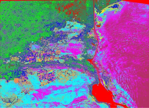 ETM 2006
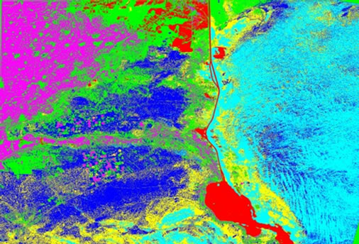 TM 1984
Figure 4. Visual results of the ISODATA classified 1984, 2006 and 2011 images.
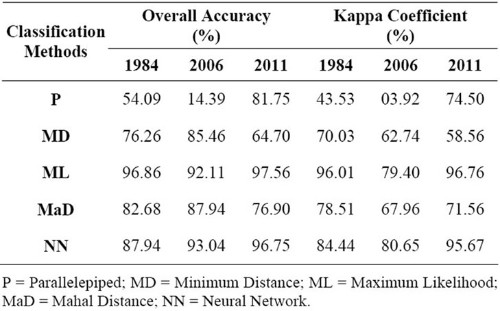
Table 2. Accuracy of different classification methods and algorithms.
4.2. Spatial Reclassification and Accuracy Assessment
With the spatial resolution refinement, the internal (spectral) variability within homogenous land-cover units is increased [49]. The increased spectral variability decreases the statistical separability of the classes in the spectral data space which reduce per-pixel classification accuracies. The resulting per-pixel classification will have a speckled (saltand-pepper effect) appearance [50]. The increased variability is attributed to the imaging of diverse class components by higher resolution sensors.
The first result of the accuracy assessment was an overall accuracy of 77% with Kappa Coefficient = 0.72. That is way bellow the “85%” cutoff level between acceptable and unacceptable result [51]. Users’ accuracies were good (above 85%). For this study, LULCC, higher accuracy was needed. The data were analyzed and reclassified again to bring this result to a wider acceptable level of accuracy. The steps for simplification were chosen based upon the classes’ similarities taken from their participation on each other in the error matrix and the qualitative justification for their misclassification.
Taking into consideration that reed vegetation in this area which is kept in a physiognomic state is very similar to “vegetation” and that it presented the lowest users accuracy in the error matrix, all reed vegetation were reclassified into “vegetation”. “Small trees” and “big trees” were the next class chosen for combination with vegetation. They had both users and producers low accuracies which can be easily explained. This procedure improved the overall accuracy. Table 3 shows the result of the land-use validation using a confusion matrix. The overall accuracy for the land-use classes was 93.04% with Kappa coefficient 80.65%. However, the question at that point is more related to the objective of the land-use mapping than to improve the accuracy.
4.3. Land-Use Change Detection, 1984-2011
At this stage, the 2006 image was not composed in further analysis due to the season of acquisition which was different from the other images. The overall accuracy of the land-use map was ranging between 96.86% and 97.56%, for the 1984 and 2011 maps respectively (Tables 2 and 3). The Kappa indices for the 1984 and 2011 maps were 0.9601 and 0.9676, respectively. Clearly, these data have a reasonable high accuracy, and thus are sufficient for land-use change detection. Table 4 shows the land-use change matrix of the Ismailia Governorate from 1984 to 2011. The prepared table shows the nature of change due to each class of the image that was obtained from the matrix algorithm, and their corresponding area in hectares. There has been a considerable change in land-use in the study area during the 27-years period.
It was possible to determine how the classes have been changed over the two dates and also the area due to each type of change (Figure 5). According to the statistics in
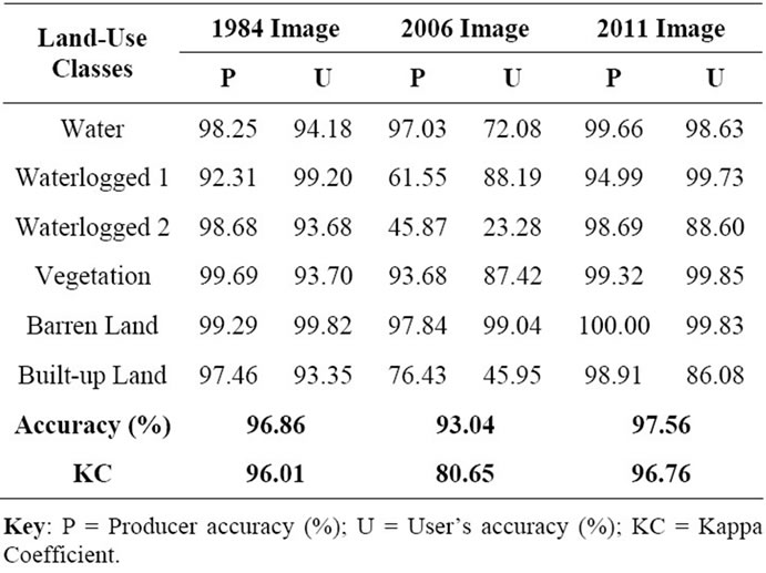
Table 3. The confusion matrix results of the land-use validation.
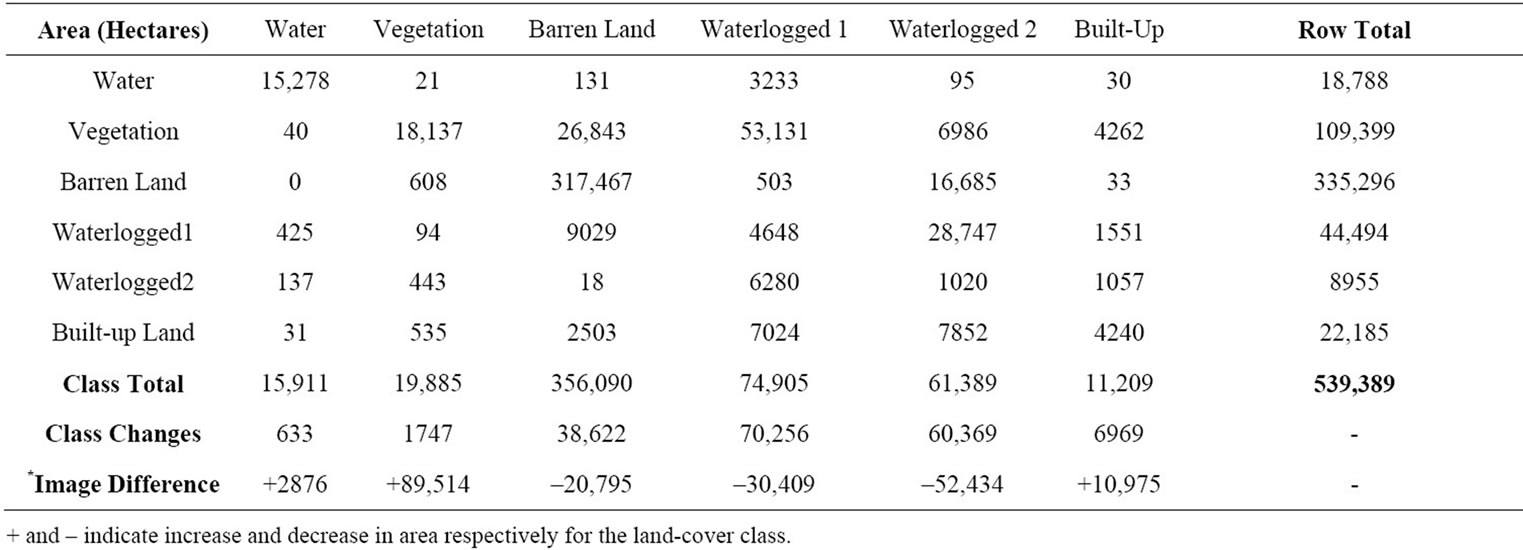
Table 4. Land-use change area representations for each Land-use for Ismailia, 1984-2011.
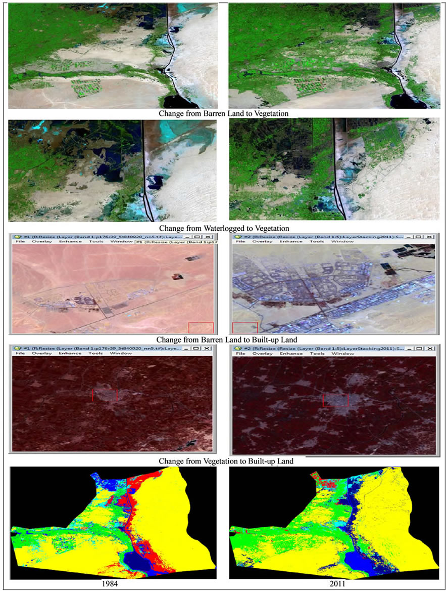
Figure 5. Areas showing significant changes in land-use types between 1984 and 2011.
Table 4 and Figure 5, it is possible to report that, vegetation class has the highest positive change (89,514 hectares) in terms of ground area in hectares. Built-up Land class has the second highest positive change (10,975 hectares). Waterlogged 2 class has undergone the highest negative change (52,434 hectares) in terms of ground area in hectares. The loss of Waterlogged 2 to the waterlogged1 class is the highest with 28,747 hectares. Waterlogged1 class has undergone the second highest negative change (30,409 hectares). Barren land class has undergone the third negative change (20,795 hectares). Barren land was also lost due to submergence by water accounting to 16,685 hectares. Due to the increasing of water table, 2876 hectares of new water bodies appear.
Based on both Table 4 and Figure 5, a change in landcover may not indicate a change in land-use. For example, field crops may be converted to fish ponds (as in Tel el-Kebir city and other areas), which constitute a change in land-cover. However, since the agriculture class does not differentiate among agriculture type, the class which includes conversion from field crops to fish ponds is a change in land-cover but not a change in land-use. Alternatively, a change in land-use may not constitute a change in land-cover. The water agriculture class represents a specific area of the Ismailia where the water is being reclaimed for crop production and fish farms (as in Abo Khalifavillage and El-Salam canal basin). This class includes water fish pond and water crops.
The water fish pond class is a change in land-use, but not a change in land-cover. Since both reservoirs and fish ponds are water bodies, so differentiating between them can be difficult, but is frequently possible because fish ponds differ in texture, tone, and size from reservoirs.
Temporarily date images may help alleviate some of the problems associated with changes due to crop phenology or the agricultural cycle that may show up as changes in land-cover but are not changes in land-use. However, anniversary date images are not always available and, even when they are available, differences in crop rotation, and phenological maturation result in changes in spectral characteristics.
4.4. Spatio-Temporal and Spectral Impact of LULCC on Surface Temperature
Table 5 summarizes the average values of radiant surface temperatures (˚C) by land-use type in 1984 and 2011. To understand the impact of LULCC on surface radiant temperature, the characteristics of the thermal signatures of each land-use type must be studied first. For both years, Urban or built-up and Barren land exhibits the highest surface radiant temperature (37.65˚C, 37.34˚C in 1984 and 43.876˚C, 42.801˚C in 2011), followed by waterlogged1 (34.54˚C in 1984 and 35.60˚C in 2011). This implies that urban development does bring up surface radiant temperature by replacing vegetation with nonevaporating surfaces such as stone, metal and concrete. The standard deviations of the radiant temperature values are small for both Built-up Land (0.55 in 1984 and 0.57 in 2011), indicating that an urban surface does not experience a wide variation in surface radiant temperature because of the dry nature ofnon-evapotranspirative materials.
The lowest radiant temperature in 1984 is observed in water (25.94˚C), followed by waterlogged 2 area (26.38˚C), and vegetation (28.73˚C). This pattern is similar with that in 2011, when the low radiant temperature is found in water (27.32˚C), followed by waterlogged2 (27.75˚C), and vegetation (32.96˚C). Vegetation shows a considerably low radiant temperature in both years, because vegetation can reduce amount of heat stored in the soil and surface through transpiration. Vegetation has low temperature because the amount of heat stored is reduced through transpiration. Vegetation land-use type is denser and the soil is not exposed. However, vegetation show a relatively large standard deviation in radiant temperature values (1.16 in 1984 and 2.81 in 2011) compared with other land-cover types, indicating the heterogeneous nature of vegetation covers. The influence of surface soil water content and vegetation contribute to a broad variation in their surface radiant temperature value. This different pattern is attributed to the differences in solar illumination, the state of vegetation, and atmospheric influences on the remotely sensed dataset.
The 1984 image was taken in 20 September while the 2011 image in 10 April. The difference in data acquisition season is clearly reflected in the surface radiant temperatures of water bodies.
The relationship between surface radiant temperature and the texture of land-cover is influenced by land-use in Ismailia Governorate. Changes in land-use can have a profound effect on the surface radiant temperature. GIS coupled with image processing can help one to visualize the impact of LULCC on surface radiant temperature. The technique of image differencing is employed to produce a radiant temperature change image after the surface radiant temperature of each year has been normalized.
The results of GIS analysis show that the urban development between 1984 and 2011 has given rise to an average increase of 6.23˚C in surface radiant temperature (Table 5 and Figure 6). On the map in Figure 6 for the Ismailia Governorate, the urban, barren land and major roads were much warmer than the rural areas covered by water. The detail in the map (Figure 6) allows one to easily locate the major roads, canals and water bodies, urban and rural areas.
The estimated surface temperature from LandSat ETM+ for 10th April was cross validated with the surface air temperature of Ismailia recorded on the same day in Ismailia Meteorological station is shown in Table 6. The difference of 6.45˚C, indicating the satellite estimation temperature is greater than the real data. This difference can be associated partly with the effects of surface roughness on surface temperature.
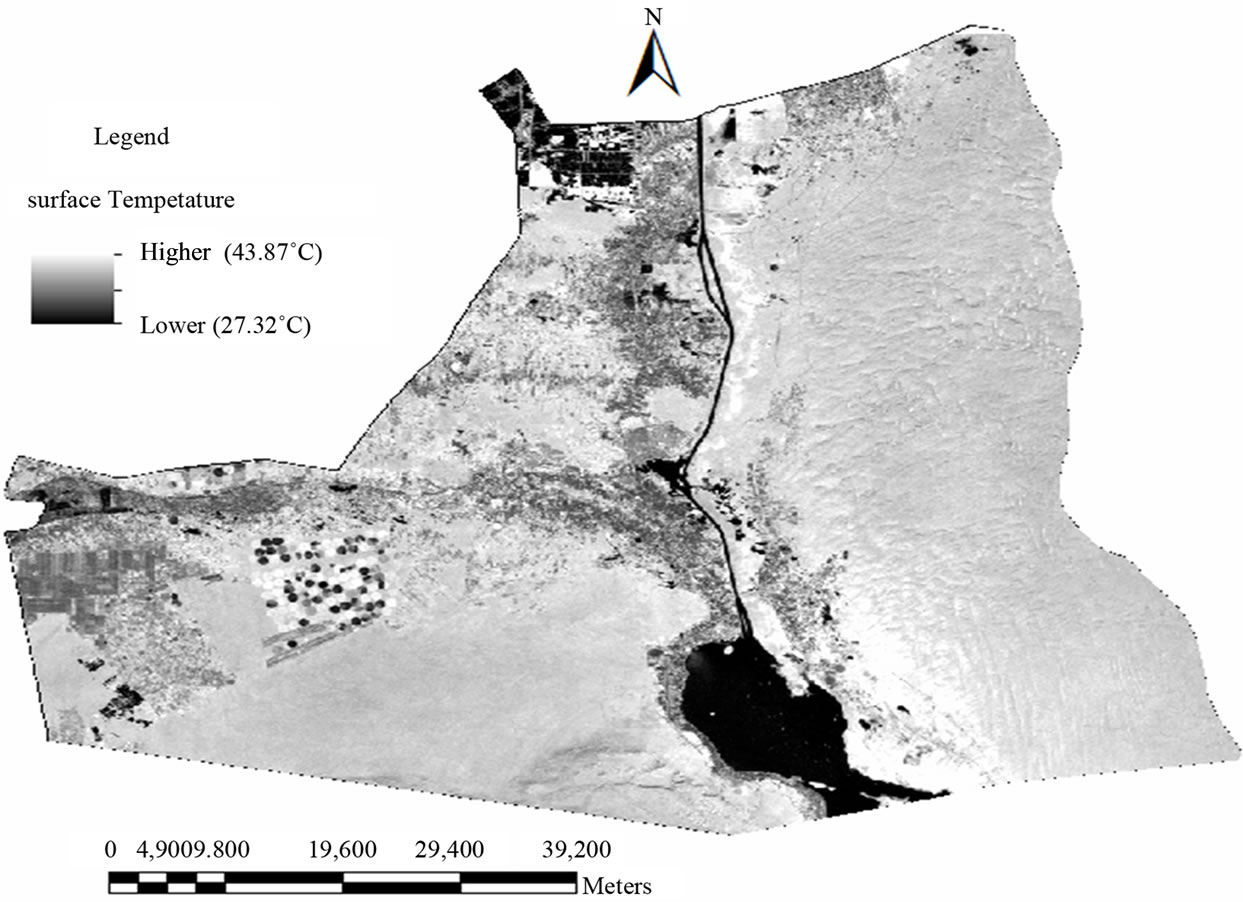
Figure 6. Image of land surface temperature for Ismailia Governorate at 10 April 2011.
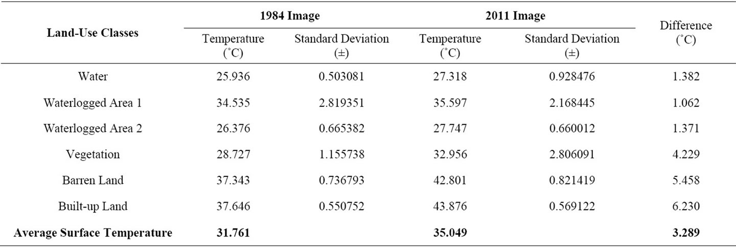
Table 5. Average surface temperature (˚C) in different land-use types.
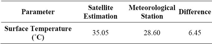
Table 6. Summary results from LandSat ETM+7 and Ismailia Meteorological station for 10th April 2011.
To conclude, thermal time-space distributions are affected by the buildings, green area and water-body on the ground, but different factors have different influences. It is very important to strengthen protecting of the city’s greening.
4.5. Relationship between Radiant Surface Temperature and NDVI
The relationship between NDVI and surface radiance temperature was studied for each land-cover type through correlation analysis (pixel by pixel). Table 7 shows the Pearson’s correlation coefficients between the two landcover in 1984 and 2011. The significance of each correlation coefficient was determined using a one tail Student’s t-test. Based on Table 7, surface radiance temperature values tend to negatively correlate with NDVI values for all land-cover types in both years. The highest NDVI was found in vegetation (0.5278, 0.6546) for the
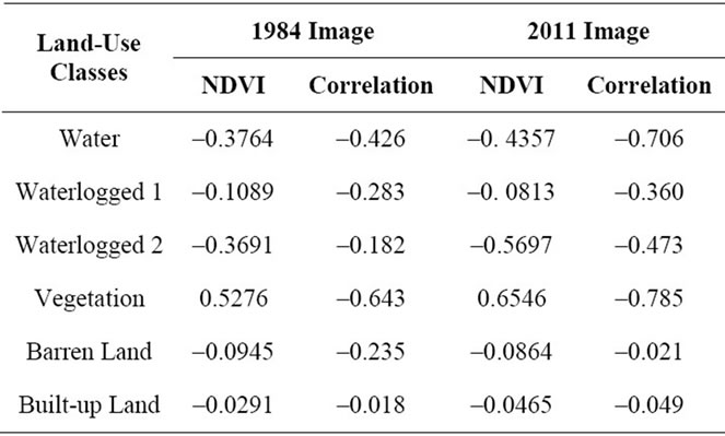
Table 7. Pearson’s correlation coefficients between average surface temperature and NDVI by land-use type (significant at 0.05 level).
1984 and 2011 images respectively. However, the lowest negative NDVI was found in urban or built-up land (–0.0291) in 1984, and (–0.0465) in 2011.
The highest negative correlation was found in vegetation (–0.643) in 1984, and (–0.785) in 2011. In both years, Built-up Land exhibits a lowest correlation (–0.018 for 1984 and –0.049 for 2011). An even lower correlation was observed in Barren Land of both years (–0.235 and –0.021) for 1984 and 2011 respectively.
To conclude, the strong negative correlation between surface radiance temperature and NDVI implies that the higher biomass a land-cover has, the lower the surface temperature. Because of this relationship between surface radiance temperature and NDVI, LULCC have an indirect impact on surface temperatures through NDVI. GIS analysis indicates that the NDVI value decreased 0.02 between 1984 and 2011 in the Built-up areas. The comparative NDVI in Ismailia falls down from 0.0291 in 1984 to 0.0465 in 2011, the reduction is 37.5%, but the temperature is rising.
4.6. Change Rate (CR) of a Land-Use Type
Table 8 shows the change rate of the major land-use types from 1984 to 2011 in Ismailia Governorate. The rate of barren land conversion to other land-use types has decreased from 1984 to 2011 by 1.12% annually. During 1984-2011, the area of water and wetland coverage increased by the annual increase of 0.82%. The increase of vegetation 0.98% area was mainly due to agriculture restructuring driven by land reclamation. In addition, due to ecological restoration waterlogged 1 and 2 decreased by 0.76, 6.61% per year.
There is a pressing need for Ismailia Governorate to use its limited land resources more efficiently and effecttively especially cultivated land. The key measures to solve the current land problems include intensive utilizetion of land resources, increasing efficiency of land-use, and enhancing environmental protection, etc.
5. Scale Dependent Land-Use Effects on Sustainable Land Management, Climate Change, and Pollution
During recent years Ismailia Governorate, has undergone the land-use changes, usually without any land evaluation for specified purposes. This leads to serious problems such as: potential agricultural failures, soil erosion, deforestation, etc. Due to increasing changes of land-use, mainly by human activities, detection of such changes, assessment of their trends and environmental effects are necessary for future planning and resource management. This leads to the following questions “Is the result obtained in the current study worth worked with for landuse management and development of the Ismailia Governorate?” and “Is the climate changing in the Ismailia Governorate?” In pressured environmentally sensitive regions, such as the Ismailia Governorate, there is a need for up-to-date and accurate land-use information that can be utilized for the analysis of environmental processes and problems for the sustainable land resources and land-use planning. Figure 7 shows the final land-use map (10/04/2011) of the Ismailia Governorate in a raster and vector format.
The aim of land-use planning in Ismailia Governorate is reusing the land in such a way that crops were cultivated in relatively large areas, reducing waste in land resources,
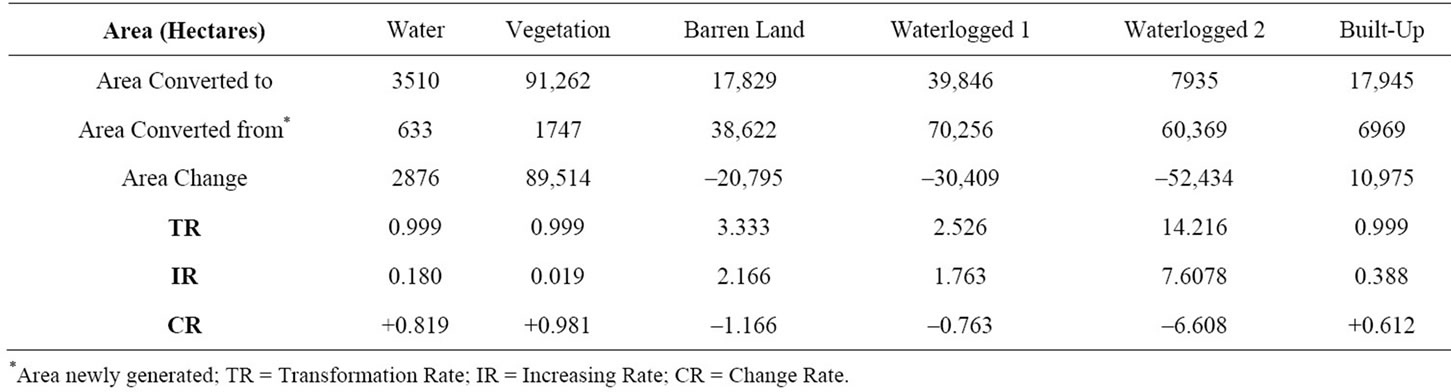
Table 8. The change rate of the major land-use types from 1984 to 2011 in Ismailia Governorate.
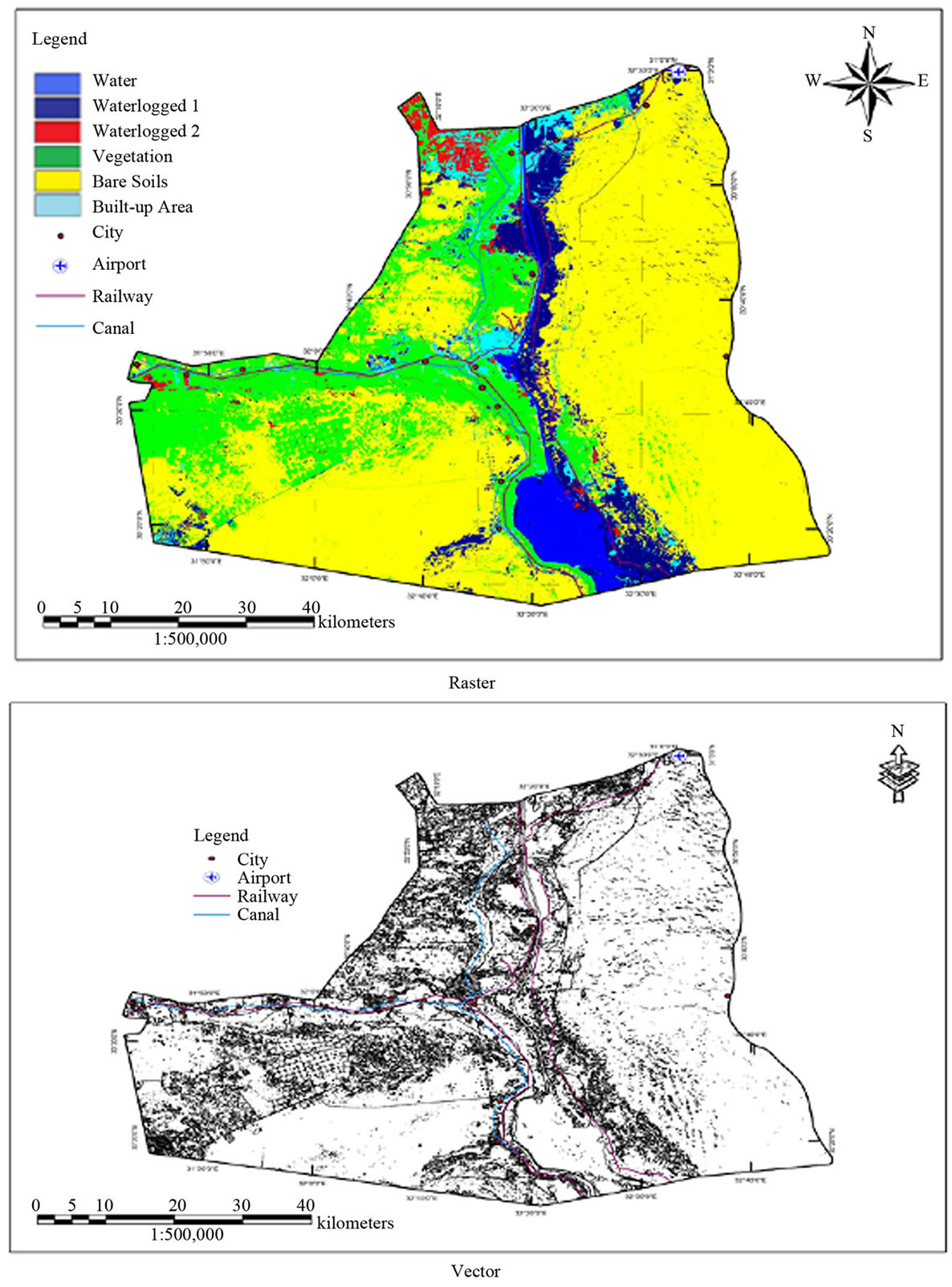
Figure 7. Final land-use map (10/04/2011) of the Ismailia Governorate in a raster and vector format.
minimizing and organizing pest control on a large scale, improving mechanical operation on the farm. However, sustainable land management is still a challenge in the Ismailia Governorate. On one hand, land management must ensure a growing supply of food and other resources to human populations, which are expected to grow for the coming decades. On the other hand, management of land to procure these resources is linked with potentially negative consequences in the form of climate change and pollution.
LULCC plays a major role in climate change in Ismailia Governorate. LULCC is responsible for releasing greenhouse gases (e.g., carbon dioxide) to the atmosphere by deforestation, especially when followed by agriculture, which causes release of soil carbon in response to disturbance by tillage. LULCC is also behind major changes in emissions of other greenhouse gases, especially methane (wetland drainage and rice paddies; cattle grazing), and nitrous oxide (agriculture: input of inorganic nitrogen fertilizers; irrigation; cultivation of nitrogen fixing plants). Land-cover changes that alter the reflection of sunlight from land surfaces (albedo) are another major driver of global climate change. These changes alter surface heat balance not only by changing surface albedo, but also by altering evaporative heat transfer caused by evapotranspiration from vegetation, and by changes in surface roughness. An example of this is the warmer temperatures observed within urban areas versus rural areas, known as the urban heat island effect which is confirmed in the current study.
LULCC is important drivers of water, soil and air pollution in Ismailia Governorate. Vegetation removal leaves soils vulnerable to massive increases in soil erosion by wind and water, especially on steep terrain. This not only degrades soil fertility over time, reducing the suitability of land for future agricultural use, but also releases huge quantities of phosphorus, nitrogen, and sediments to canals and surface water causing negative impacts (increased sedimentation and turbidity). Intensive agricultural inputs of nitrogen and phosphorus fertilizers have been increased the pollution of surface water by runoff and erosion and the pollution of groundwater by leaching of excess nitrogen. Other agricultural chemicals, includeing herbicides and pesticides are also released to ground and surface water by agriculture and in some cases remain as contaminants in the soil. The burning of vegetation biomass (crop residues, weeds) to clear agricultural fields remains a potent contributor to air pollution wherever it occurs.
6. Concluding Remarks and Limitations
This study introduces a methodology using combination of RS/GIS techniques to update land-use change data base. The data base contains detailed information on the spatial distribution of main agricultural crops, water, waterlogged areas, barren land, and built-up areas. The present study shows that RS/GIS based land-use mapping is very effective. The Landsat TM/ETM satellite is good source to provide information accurately. The Maximum Likelihood classification method proved to be very efficient to classify land-cover over Ismailia Governorate, Egypt. Six land-use/land-cover classes (urban, vegetation, waterlogged 1 and 2, bare land, and water) are identified. An overall accuracy and overall Kappa higher than 80% were achieved. Urban or built-up and Barren land exhibits the highest surface radiant temperature, followed by waterlogged1 and vegetation.
The lowest radiant temperature in 1984 is observed in water, followed by waterlogged area 2. This pattern is similar with that in 2011. This different pattern is attributed to the differences in solar illumination, the state of vegetation, and atmospheric influences on the remotely sensed dataset. The highest NDVI was found in vegetation for the 1984 and 2011 images. However, the lowest negative NDVI was found in urban or built-up land in 1984 and 2011. In both years, Built-up Land exhibits a lowest correlation. An even lower correlation was observed in Barren Land of both years.
The change rates of the major land-use types from 1984 to 2011 which are decreased are barren land (1.12% annually) and waterlogged1 and 2 (0.76% and 6.61% annually). However, the vegetation, water, and built-up areas are increased by 0.98%, 0.82%, and 0.61% per year, respectively. The results show that the database containing information on actual land-use is necessary for various applications, such as land evaluation, soil erosion, and desertification. The spatial, temporal, and spectral characteristics of the remote sensing data are effectively used in land-use and land-cover change mapping in the current study, hence helping in decision making for sustainable land resource management. This methodology should be applied to other regions in Egypt.
This paper suggests three limitations to this research that need to be addressed in the future. First, the computed surface radiant temperatures may be different than as they were, since the effects of surface roughness on surface temperature have not been taken into account. Second, the resolution of the images can affect the classification accuracy and detecting changes in land features. For example, it may be difficult to distinguish different agricultural lands (e.g., crops, vegetables…). Third, many land-use types were identified in this study. Waterlogged and Gypsiferous soils are one of these types that show higher temperature than expected.
These (Gypsiferous) soils may be agriculturally important for future generations. These soils can be converted to agricultural land. So the future research can answer the question “Are pedologists overlooking unconventional soil science?” Till now, a limited progress has been made in this direction.
7. Acknowledgements
The author would like to thank Prof. Dr. M. Reda and Miss. S. M. Reda for their helpful reviews of this paper.
REFERENCES
- G. Kirk, “Views on the Future of Soil Science,” In: A. Hartemink, Ed., The Future of Soil Sciences, International Union of Soil Sciences, 2006.
- El. E. Omran, “Is Soil Science Dead and Buried? Future Image in the World of 10 Billion People,” CATRINA, Vol. 3, No. 2, 2008, pp. 59-68.
- W. N. Adger, N. W. Arnell and E. L. Tompkins, “Successful Adaptation to Climate Change across Scales,” Global Environmental Change, Vol. 15, No. 2, 2005, pp. 77-86. doi:10.1016/j.gloenvcha.2004.12.005
- E. Erle and P. Robert, “Land-Use and Land-Cover Change,” In: J. C. Cutler, Ed., Encyclopedia of Earth, Environmental Information Coalition, National Council for Science and the Environment, Washington DC, 2010.
- J. A. Foley, R. DeFries, G. P. Asner, C. Barford and G. Bonan, “Global Consequences of Land Use,” Science, Vol. 309, No. 5734, 2005, pp. 570-574. doi:10.1126/science.1111772
- J. K. Parikh and K. Parikh, “Climate Change: India’s Perceptions, Positions, Policies and Possibilities,” India Gandhi Institute of Development Research, 2002. http://www.oecd.org/dataoecd/22/16/1934784.pdf
- UNFCCC, “Climate Change: Impacts, Vulnerabilities and Adaptation in Developing Countries,” United Nations Framework Convention on Climate Change, 2007. http://unfccc.int/resource/docs/publications/impacts.pdf
- El. E. Omran, “A Proposed Simplified Method to Improve Land-Use Mapping Accuracy,” Agricultural Research Journal, Vol. 9, No. 3, 2009, pp. 123-132.
- R. Manonmani and D. S. Mary, “Remote Sensing and GIS Application in Change Detection Study in Urban Zone Using Multi Temporal Satellite,” International Journal of Geomatics and Geosciences, Vol. 1, No. 1, 2010.
- V. G. Pece, “Assessment of Land Use and Land Cover Changes around Ohrid and Prespa Lakes Using Landsat Imagery,” BALWOIS, Ohrid, Republic of Macedonia, 2008.
- Z. Qiming, L. Baolin and S. Bo, “Modelling SpatioTemporal Pattern of Landuse Change Using Multi-temporal Remotely Sensed Imagery,” The International Archives of the Photogrammetry, Remote Sensing and Spatial Information Sciences, Vol. XXXVII, Part B7, 2008.
- R. Selçuk, “Analyzing Land Use/Land Cover Changes Using Remote Sensing and GIS in Rize, North-East Turkey,” Sensors, Vol. 8, No. 10, 2008, pp. 6188-6202. doi:10.3390/s8106188
- M. T. Wubet, “Estimation of Absolute Surface Temperature by Satellite Remote Sensing,” M.Sc Thesis, International Institute for Geoinformation Science and Earth Observation, Netherlands, 2003.
- R. C. Balling and S. W. Brazell, “High Resolution Surface Temperature Patterns in a Complex Urban Terrain,” Photogrammetric Engineering & Remote Sensing, Vol. 54, No. 9, 1988, pp. 1289-1293.
- K. P. Gallo, A. L. McNab, T. R. Karl, J. F. Brown, J. J. Hood and J. D. Tarpley, “The Use of NOAA AVHRR Data for Assessment of the Urban Heat Island Effect,” Journal of Applied Meteorology, Vol. 32, No. 5, 1993, pp. 899-908. doi:10.1175/1520-0450(1993)032<0899:TUONAD>2.0.CO;2
- S. Q. Kidder and H. T. Wu, “A Multispectral Study of the St. Louis Area under Snow Covered Conditions Using NOAA-7 AVHRR Data,” Remote Sensing of Environment, Vol. 22, No. 2, 1987, pp. 159-172. doi:10.1016/0034-4257(87)90056-3
- M. Roth, T. R. Oke and W. J. Emery, “Satellite Derived Urban Heat Islands from Three Coastal Cities and the Utilisation of Such Data in Urban Climatology,” International Journal of Remote Sensing, Vol. 10, No. 11, 1989, pp. 1699-1720. doi:10.1080/01431168908904002
- W. H. Carnahan and R. C. Larson, “An Analysis of an Urban Heat Sink,” Remote Sensing of Environment, Vol. 33, No. 1, 1990, pp. 65-71. doi:10.1016/0034-4257(90)90056-R
- Q. Weng, “Fractal Analysis of Satellite-Detected Urban Heat Island Effect,” Photogrammetric Engineering & Remote Sensing, Vol. 69, No. 5, 2003, pp. 555-566.
- Q. Weng, “Thermal Infrared Remote Sensing for Urban Climate and Environmental Studies: Methods, Applications, and Trends,” ISPRS Journal of Photogrammetry and Remote Sensing, Vol. 64, No. 4, 2009, pp. 335-344. doi:10.1016/j.isprsjprs.2009.03.007
- M. Reda and El. E. Omran, “Strategy for the Exploitation of Land Resources to Ismailia Governorate until 2017,” 1997 (Unpublished Report).
- F. Sabins, “Remote Sensing: Principles and Interpretation,” WH Freeman & Co., New York, 1996.
- A. Almutairi and A. T. Warner, “Change Detection Accuracy and Image Properties: A Study Using Simulated Data,” Remote Sensing, Vol. 2, No. 6, 2010, pp. 1508- 1529. doi:10.3390/rs2061508
- P. C. Alexandre and W. Eleonore, “Change Detection for Updates of Vector Database through Region-Based Classification of VHR Satellite Data,” Proceedings of SPIE, Vol. 6749, 2007, p. 11.
- J. Gong, H. Sui, G. Ma and Q. Zhou, “A Review of Multi-Temporal Remote Sensing Data Change Detection Algorithms,” The International Archives of the Photogrammetry, Remote Sensing and Spatial Information Sciences, Vol. XXXVII, Part B7, 2008.
- A. Singh, “Digital Change Detection Techniques Using Remotely Sensed Data,” International Journal of Remote Sensing, Vol. 10, No. 6, 1989, pp. 989-1003. doi:10.1080/01431168908903939
- D. Yuan, C. D. Elvidge and R. S. Lunetta, “Survey of MULTISPECTRAL Methods for Land Cover Change Analysis,” In: R. S. Lunetta and C. D. Elvidge, Eds., Remote Sensing Change Detection: Environmental Monitoring Methods and Applications, Taylor & Francis, London, 1999, pp. 21-39.
- G. Chander, B. L. Markham and D. L. Helder, “Summary of Current Radiometric Calibration Coefficients for Landsat MSS, TM, ETM+, and EO-1 ALI Sensors,” Remote Sensing of Environment, Vol. 113, No. 5, 2009, pp. 893-903. doi:10.1016/j.rse.2009.01.007
- K. P. Gallo, A. L. McNab, T. R. Karl, J. F. Brown, J. J. Hood and J. D. Tarpley, “The Use of a Vegetation Index for Assessment of the Urban Heat Island Effect,” International Journal of Remote Sensing, Vol. 14, No. 11, 1993, pp. 2223-2230. doi:10.1080/01431169308954031
- R. R. Gillies and T. N. Carlson, “Thermal Remote Sensing of Surface Soil Water Content with Partial Vegetation Cover for Incorporation into Climate Models,” Journal of Applied Meteorology, Vol. 34, 1995, pp. 745-756. doi:10.1175/1520-0450(1995)034<0745:TRSOSS>2.0.CO;2
- C. T. Kok, S. L. Hwee, Z. M. Mohd and A. Khiruddin, “Landsat Data to Evaluate Urban Expansion and Determine Land Use/Land Cover Changes in Penang Island, Malaysia,” Environmental Earth Sciences, Vol. 60, No. 7, 2010, pp. 1509-1521. doi:10.1007/s12665-009-0286-z
- K. R. Martha, C. C. Josefino, A. W. Donald and V. David, “Relationship between Satellite-Derived Land Surface Temperatures, Arctic Vegetation Types, and NDVI,” Remote Sensing of Environment, Vol. 112, No. 4, 2008, pp. 1884-1894. doi:10.1016/j.rse.2007.09.008
- W. Qihao, L. Dengsheng and S. Jacquelyn, “Estimation of Land Surface Temperature-Vegetation Abundance Relationship for Urban Heat Island Studies,” Remote Sensing of Environment, Vol. 89, No. 4, 2004, pp. 467-483. doi:10.1016/j.rse.2003.11.005
- A. H. S. Salah, “Remote Sensing and GIS Techniques for Urban Growth Monitoring of Basarah City,” International Journal of Remote Sensing and Earth Sciences, Vol. 7, 2010, pp. 73-83.
- H. L. Long, G. K. Heilig, X. B. Li and M. Zhang, “SocioEconomic Development and Land-Use Change: Analysis of Rural Housing Land Transition in the Transect of the Yangtse River, China,” Land Use Policy, Vol. 24, No. 1, 2007, pp. 141-153. doi:10.1016/j.landusepol.2005.11.003
- H. L. Long, Y. S. Liu, X. Q. Wu and G. H. Dong, “Spatio-Temporal Dynamic Patterns of Farmland and Rural Settlements in Su-Xi-Chang Region: Implications for Building a New Countryside in Coastal China,” Land Use Policy, Vol. 26, No. 2, 2009, pp. 322-333. doi:10.1016/j.landusepol.2008.04.001
- J. Wang, Y. Chen, X. Shao, Y. Zhang and Y. Cao, “LandUse Changes and Policy Dimension Driving Forces in China: Present, Trend and Future,” Land Use Policy, Vol. 29, No. 4, 2012, pp. 737-749. doi:10.1016/j.landusepol.2011.11.010
- El. E. Omran, “Evaluation of the Egyptian Soil Maps Accuracy,” Egyptian Journal of Soil Sciences, 2012, In Press.
- R. G. Congalton, “A Review of Assessing the Accuracy of Classifications of Remotely Sensed Data,” Remote Sensing of Environment, Vol. 37, No. 1, 1991, pp. 35-46. doi:10.1016/0034-4257(91)90048-B
- T. M. Lillesand and R. W. Kiefer, “Remote Sensing and Image Interpretation,” John Wiley & Sons Inc., New York, 2000.
- L. F. Janssen and W. J. Vander, “Accuracy A Review,” Photogrammetric Engineering & Remote Sensing, 1994, pp. 419-425.
- J. L. Van Genderen, B. F. Lock and P. A. Vass, “Remote Sensing: Statistical Testing of Thematic Map Accuracy,” Remote Sensing of Environment, Vol. 7, No. 1, 1978, pp. 3-14. doi:10.1016/0034-4257(78)90003-2
- J. F. Anderson, E. E. Hardy, J. T. Roach and R. E. Witmer, “A Land Use and Land Cover Classification System for Use with Remote Sensor Data,” U.S. Geological Survey Professional Paper 964, US Geological Survey, Washington DC, 1976, p. 28.
- H. Y. Araya and P. Cabral, “Analysis and Modeling of Urban Land Cover Change in Setúbal and Sesimbra, Portugal,” Remote Sensing, Vol. 2, 2010, pp. 1549-1563.
- F. Bektas, “Remote Sensing and Geographic Information Integration: A Case Study, Bozcaada &Gokceada Island,” M.Sc Thesis, Institution of Science and Technology, Istanbul Technical University, 2003.
- ESRI, “ArcMap Version 9.3 User Manual,” Redlands, CA, USA, 2008.
- D. J. Booth and R. B. Oldfield, “A Comparison of Classification Algorithms in Terms of Speed and Accuracy after the Application of a Post Classification Modal Filter,” International Journal of Remote Sensing, Vol. 10, No. 7, 1989, pp. 1271-1276. doi:10.1080/01431168908903965
- S. K. Alvipanah and M. Masoudi, “Land Use Mapping Using Land Sat TM Data and GIS (Case Study: Mouk Area, Iran),” Journal of Agricultural Science and Natural Resources, Vol. 8, No. 1, 2001.
- A. P. Carleer, O. Debeir and E. Wolff, “Assessment of Very High Spatial Resolution Satellite Image Segmentations,” Photogrammetric Engineering & Remote Sensing, Vol. 71, No. 11, 2005, pp. 1285-1294.
- G. M. Smith and R. M. Fuller, “An Integrated Approach to Land Cover Classification: An Example in the Island of Jersey,” International Journal of Remote Sensing, Vol. 22, No. 16, 2001, pp. 3123-3142. doi:10.1080/01431160152558288
- R. G. Congalton and K. Green, “Assessing the Accuracy of Remotely Sensed Data: Principles and Practices,” Lewis Publisher, Boca Raton, 1999.