Natural Science
Vol.6 No.7(2014), Article ID:45337,12 pages DOI:10.4236/ns.2014.67044
Weighted Gini-Simpson Quadratic Index of Biodiversity for Interdependent Species
Radu Cornel Guiasu1, Silviu Guiasu2
1Environmental and Health Studies Program, Department of Multidisciplinary Studies, Glendon College, York University, Toronto, Canada
2Department of Mathematics and Statistics, York University, Toronto, Canada
Email: rguiasu@glendon.yorku.ca, guiasus@pascal.math.yorku.ca
Copyright © 2014 by authors and Scientific Research Publishing Inc.
This work is licensed under the Creative Commons Attribution International License (CC BY).
http://creativecommons.org/licenses/by/4.0/


Received 31 December 2013; revised 31 January 2014; accepted 7 February 2014
ABSTRACT
The weighted Gini-Simpson quadratic index is the simplest measure of biodiversity which takes into account the relative abundance of species and some weights assigned to the species. These weights could be assigned based on factors such as the phylogenetic distance between species, or their relative conservation values, or even the species richness or vulnerability of the habitats where these species live. In the vast majority of cases where the biodiversity is measured the species are supposed to be independent, which means that the relative proportion of a pair of species is the product of the relative proportions of the component species making up the respective pair. In the first section of the paper, the main versions of the weighted Gini-Simpson index of biodiversity for the pairs and triads of independent species are presented. In the second section of the paper, the weighted Gini-Simpson quadratic index is calculated for the general case when the species are interdependent. In this instance, the weights reflect the conservation values of the species and the distribution pattern variability of the subsets of species in the respective habitat induced by the inter-dependence between species. The third section contains a numerical example.
Keywords:Weighted Gini-Simpson Index, Generalized Rao Index, Interdependent Species, Watanabe’s Entropic Measure of Interdependence, Distribution Pattern Variability of the Subsets of Species

1. Introduction
In a certain habitat, let  be the number of species;
 ![]() the relative abundance of species
the relative abundance of species![]() ;
;  the distribution of the relative abundance of species. We have:
The simplest measure of biodiversity is the Gini-Simpson quadratic index (Gini [1] , Simpson [2] ):
![]()
Recently, Jost [3] [4] , and Jost et al. [5] gave some examples showing that the Gini-Simpson index does not behave well when the number of species n is very large. Guiasu and Guiasu [6] showed, however, that the Rich-Gini-Simpson index:
![]() which depends explicitly on the number of species (species richness), preserves all the properties of the classic Gini-Simpson index GS but, unlike GS, behaves very well when n is large.
which depends explicitly on the number of species (species richness), preserves all the properties of the classic Gini-Simpson index GS but, unlike GS, behaves very well when n is large.
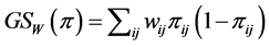
Another measure of diversity is the weighted Gini-Simpson index introduced in Guiasu and Guiasu [7] :
![]() where
where  are some nonnegative weights assigned to the species, such as the conservation values of the respective species, for instance. Obviously,
  becomes RGS if
  for each
Let us assume that in a certain region there are  species and
  sites. In what follows, the subscripts
 ![]() and
and  refer to species
  and the subscripts
  and
and  refer to sites,
 .
.
Let  be the vector whose components are the relative abundances of the individual species within site
 , such that:
![]()
for each  A measure of diversity μ may be used in the standard additive partioning of diversity induced by individual species if it is a concave function, which means that it satisfies the inequality:
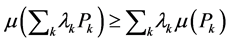 (1)
(1)
for arbitrary parameters:
![]() (2)
(2)
For each site , we calculate the diversity
  among its species, called the local diversity of the respective site. In such a case, as pointed out by Lande [8] , the right-hand side of (1) is the α-diversity, denoted by α, measuring the average local diversity, or the average within-diversity. The left-hand side of (1) is the γ-diversity, denoted by γ, measuring the diversity among the species belonging to the averaged union of the habitats, called the regional or total diversity. As shown in [6] [7] [9] , the measures of biodiversity
![]() ,
, ![]() , and
, and , the last one when its weights do not depend on the relative proportions of species
 , are concave functions and satisfy the inequality (1), for arbitrary parameters (2). Unlike the α-diversity and the γ-diversity, there is no consensus about how to interpret and calculate the β-diversity. According to Whittaker [10] [11] who introduced the terminology, β-diversity is the ratio between γ-diversity and α-diversity, namely,
 . This is the multiplicative partitioning of diversity. According to MacArthur [12] , MacArthur and Wilson [13] , and Lande [8] , β-diversity is the difference between γ-diversity and α-diversity, namely,
 . This is the additive partitioning of diversity. In both cases, the β-diversity measures the variation of the diversity among habitats, or the average between-diversity in the additive case.
As the classic Gini-Simpson index ![]() is a concave function of the relative abundance of species
is a concave function of the relative abundance of species , it may be used in the additive partitioning of diversity. Hill [14] showed that:

may be used in the multiplicative partitioning of diversity. Similarly, the weighted Gini-Simpson quadratic index  is a concave function of the relative abundance of species
  if the weights
  do not depend on the relative abundance
  and, therefore, may be used in the additive partitioning of diversity, where
 . The corresponding multiplicative weighted Gini-Simpson quadratic index for individual species:
may be used in the multiplicative partitioning of diversity where the  -diversity is the ratio between the
 ![]() - diversity and the α -diversity, i.e.
- diversity and the α -diversity, i.e. .
.
Let  be a square matrix whose entries are the distances between species, such as the phylogenetic distances, for instance. Thus,
  is the distance between the species
 ![]() and
and , and we have:
 .
.
Rao’s index [15] , also called quadratic entropy or dissimilarity measure, is:
Viewed as a function of the relative abundance of individual species,  is a quadratic function. Unfortunately, if the distance matrix
 ![]() is arbitrary, Rao’s index
is arbitrary, Rao’s index , taken as a diversity measure μ, does not satisfy the inequality (1) for arbitrary parameters (2) and, therefore, cannot be used in a standard additive partitioning of the diversity. There are some excellent papers dealing with diversity (Pavoine et al. [16] , Ricotta [17] , Ricotta and Szeidel [18] , Hardy and Senterre [19] , Villéger and Mouillot [20] , Hardy and Jost [21] , Ricotta and Szeidel [22] , Sherwin [23] , De Bello et al. [24] , and Tuomisto [25] [26] ). Some of them discuss how to use Rao’s index
  in the additive partioning of diversity. Some research focused on finding special kinds of distance matrices D for which the corresponding Rao’s index
  is a concave function, such as the matrix
  assumed to be Euclidean, for instance. Some other research focused on how to use Rao’s index for getting a nonstandard additive partitioning of diversity, which means determining whether some special parameters (2) could be used in order to define analog α-, β-, and γ-diversities corresponding to these particular parameters. However, the weighted Gini-Simpson quadratic index of biodiversity, applied to the pairs of species, provides a concave replacement of Rao’s index and, therefore, is appropriate for use in the additive partitioning of diversity for arbitrary distance matrix
![]() .
.
Let  be the weight assigned to the pair of species
 ;
;  is the joint probability of the ordered pair of species
 . The joint probability of the pair of species
  is:
is: . We have:
Denote by:  and
and . Let
. Let  be the value of species
 ![]() and
and . Again, let
  be the matrix whose entry
  is the distance between the species
 ![]() and
and . The weighted GiniSimpson quadratic index of biodiversity for pairs of species is:
 .
.
As shown in Guiasu and Guiasu ([27] [28] ),  is a concave function of the joint distribution
 , when the weights do not depend on the probability distribution
 , and, therefore, may be used in the additive partitioning of diversity, where
 . The corresponding multiplicative weighted Gini-Simpson quadratic index for pairs of species:
 ;
;
may be used in the multiplicative partitioning of diversity where the  -diversity is the ratio between the
 ![]() - diversity and the
- diversity and the  -diversity, i.e.
 .
.
Let us assume now that the weights are:
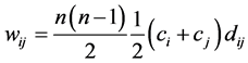 where:
  is the number of distinct pairs of species (the richness of the distinct pairs of species), and
  is the average value of the pair of species
 . If the species are considered to be independent from the point of view of their relative abundance, then:
 and the corresponding weighted Gini-Simpson quadratic index of biodiversity for the distinct pairs of species becomes:
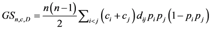 .
.
As mentioned in [27] [28] , this measure is a concave replacement of the Rao’s index. It depends on the distance between species, the richness of the pairs of distinct species, the value of the species, and the relative proportion of the species.
As shown in [9] , the weighted Gini-Simpson quadratic index may be applied to the study of the biodiversity of the triads of species as well. Let  be the matrix whose generic entry
  is the distance between species
 ![]() and
and . The area of the triangle formed by the distinct species
![]() ,
,  , and
, and , is given by the Heron’s formula:
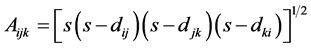 where
where  is the semi-perimeter of this triangle:
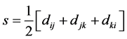 .
.
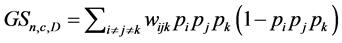
If the species are independent from the point of view of their relative abundance, taking  and the richness of the triads of species as weights, the corresponding weighted Gini-Simpson quadratic index for triads of independent species is:
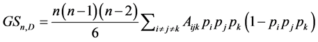 where
where 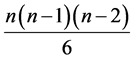 is the number of distinct triads of species. If the values of the species are also taken into account, the weighted Gini-Simpson quadratic index for triads of species is:
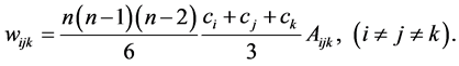
 where the weights are:
2. Interdependent Species
In the current literature on biodiversity the species from a habitat are considered to be independent from the point of view of their relative abundance and the separate abundance of each species is taken into account. Thus, if ![]() is the relative proportion of species
is the relative proportion of species![]() , then the relative proportion of the ordered pair of species
, then the relative proportion of the ordered pair of species  is
is . In real life, however, the species can be interdependent and the biodiversity in the ecosystem is influenced by this interdependence. For instance, pairs of species can interact in various types of inter-specific ecological relationships, including mutualism, where both species benefit from the interaction, commensalism, where one species benefits and the other one is not significantly affected, and parasitism, where the parasite benefits and the host species is harmed. While interactions between pairs of species are easier to study, and have generally been the focus of most inter-specific studies, the interdependence among several species within a particular ecosystem can often be much more complex and crucial for determining the biodiversity found at a certain location. As an example, in sage-scrub habitat fragments in southern California, the presence of coyotes (the top predators in these habitats) keeps the numbers of mesopredators, such as domestic cats and raccoons, down. Since domestic cats are effective predators of local scrub-breeding birds, these bird species actually benefit from the presence of coyotes. Therefore, when the coyote populations decline, local scrub-breeding birds are more likely to become extinct, and bird species diversity decreases (Crooks and Soulé [29] ). This is an example of multiple interactions involving several species, which shows how these inter-specific relationships can affect the biodiversity of the ecosystem.
Let  be the distinct species that may be found in a given large habitat, like some species of plants on a large island, for instance. Making observations at several different locations of this island, denote by
  the number of locations where only the species
  have been found, coexisting together. If
 ![]() is the total number of locations where observations have been made, the relative proportion of the subset of species
is the total number of locations where observations have been made, the relative proportion of the subset of species  is:
is:
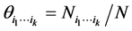 .
.
We have:
 where
where ![]() is the relative proportion of finding none of the species
is the relative proportion of finding none of the species  at the locations on the island where observations have been made.
Let  be some nonnegative weights assigned to the subset of species
 . The weighted GiniSimpson quadratic index for interdependent species is:
 . (3)
. (3)
The main problem is to investigate what kind of weights could adequately reflect the species biodiversity on the island, along with the abundance of these species. A reasonable answer is offered by the use of Shannon’s [30] entropy, as a measure of uncertainty, and Watanbe’s [31] entropic measure of interdependence.
As mentioned before,  is the relative abundance of the separate subset of species
  alone, or the probability of finding only the subset of species
 , and no other species, at a location on the island where observations have been made. Let
  be the probability distribution that describes the presence, denoted by the symbol 1, or absence, denoted by the symbol 0, of the species belonging to the subset
 . The Shannon entropy
  corresponding to the probability distribution
  measures how much variability is induced on the respective island by the subset of species
  at the locations where observations have been made. The subset of species
  contributes more to the diversity of the respective habitat if its variability, as measured by the corresponding entropy
 , is larger. We have:
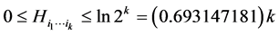 .
.
The minimum value corresponds to the case when the same configuration present/absent of the species of the subset  is found at every location where observations were made. This happens, for instance, when all the species of the subset
  were found at every location. In such a case, there is no variability as far as the distribution of the subset of species
  on the respective island is concerned. The maximum value corresponds to the case when all the configurations indicating presence/absence of the species from the subset
  are encountered at the different locations where observations were made, with equal likelihood, thereby inducing a maximum variability on the island.
For the subset , the components of the probability distribution
 , which describes its distribution pattern variability, are
  and
and  giving the probability that the species
  is present or absent at the locations where observations were made. The corresponding entropy is:
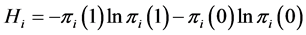 .
.
We have:  where the minimum is obtained when
 , which means that the species
  is present, with certainty, at every location, or when
 , which means that the species
  is absent, with certainty, at every location. In both such cases, the species
  induces no distribution variability on the island. The maximum value of
  corresponds to the case when
 , which means that the species
  is present at half of the locations and absent at the other half, inducing a maximum variability on the island. This has nothing to do with the abundance of the species
 , which obviously contributes to the diversity on the island; it has to do with the way in which the species
  is distributed within the respective island. Abundance and distribution variability are both components of diversity.
For the subset , the components of the probability distribution
 , which describes its distribution pattern variability, are
 ,
,  ,
,  and
and , giving the probability that the species
  and
and ![]() are present or absent at the locations where observations were made. Thus,
are present or absent at the locations where observations were made. Thus,  , for instance, is the probability that both species are present, or proportion of locations where both
  and
and ![]() are present. The corresponding entropy is:
are present. The corresponding entropy is:
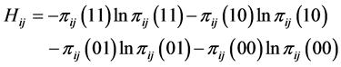 .
.
We have: ![]() where the minimum is obtained when
where the minimum is obtained when , or when
 , or when
 , or when
 , which means that only one of the patterns 11, 10, 01, or 00 is observed, with certainty, at every location. This indicates that the subset of species
  induces no distribution pattern variability on the respective island. The maximum value of
  corresponds to the case when
 . This indicates that the four different patterns of presence/absence of the two species are uniformly distributed at the locations on the island where observations were made, inducing a maximum distribution pattern variability on the island.
If the species of the subset  were independent, as far as the individual presence/absence is concerned, then the entropy
  would be a suitable weight reflecting the distribution pattern variability induced by this subset of species. But, more often than not, the species are not independent as far as the individual presence/absence is concerned. The interdependence between species will diminish variability. To give a simple example, if two species,
  and
and![]() , are independent, as far as the individual presence/absence is concerned, then there are four possibilities to consider at each location: (a)
, are independent, as far as the individual presence/absence is concerned, then there are four possibilities to consider at each location: (a)  present and
 ![]() present; (b)
present; (b)  present and
 ![]() absent; (c)
absent; (c)  absent and
 ![]() present; (d)
present; (d)  absent and
 ![]() absent. If, however, the two species are interdependent and, for instance, can be present only together, then there are only two possibilities to deal with, namely: (a)
absent. If, however, the two species are interdependent and, for instance, can be present only together, then there are only two possibilities to deal with, namely: (a)  present and
 ![]() present; (b)
present; (b)  absent and
 ![]() absent. Obviously, we have less variability due to the interdependence between the two species.
absent. Obviously, we have less variability due to the interdependence between the two species.
The amount of interdependence between the species of the subset , as introduced by Watanabe [31] , is given by the sum of the entropies of the species of the subset minus the entropy of the entire subset of species, namely:
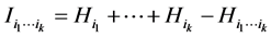 .
.
We have: , and
, and  if and only if the species of the subset
  are independent. Details may be found in Guiasu [32] .
The degree of distribution pattern variability induced by the subset of species  on the respective island is obtained by subtracting the interdependence between the species of the subset
  from the entropy of this subset of species, namely:
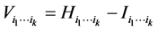 .
.
Summarizing, diversity depends on the abundance of species, the number of species (richness), the values of species, and the distribution pattern variability of the species. The classic Gini-Simpson index measures diversity taking into account only the abundance of species. The weighted Gini-Simpson quadratic index takes into account all four factors just mentioned.
Let  be the positive numbers reflecting the value of the species
 , respectively, such as the conservation values of species, for instance. Normally,
 . The weight assigned to the subset of species
  is:
is:
 . (4)
. (4)
Obviously,  and
and , because:
 ;
; .
.
If we do not take the value of the species into account or have no such information available, then we assume that , in which case
 , which is the richness of the subset of species
  , and the weights (4) become:
 .
.
The main conclusion is that for interdependent species, the diversity is measured by the formula (3) where the weights are given by (4).
3. Numerical Example
On an island, observations are made at several locations, looking for four species of plants, denoted by . Seven different patterns have been found, denoted by
 , as shown in the table below, with the relative frequencies:
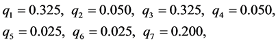
respectively.
|
|
|
|
|
|
|
| |
|
| 1 | 1 | 1 | 1 | 0 | 0 | 0 |
|
| 1 | 1 | 0 | 0 | 1 | 1 | 0 |
|
| 0 | 0 | 1 | 1 | 1 | 1 | 0 |
|
| 0 | 1 | 0 | 1 | 0 | 1 | 1 |


The entries in this table are: 1 meaning “presence” and 0 meaning “absence” of the species from the rows in the patterns from the columns. Thus, pattern![]() , for instance, shows that the species
, for instance, shows that the species 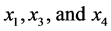 have been found together at a certain location, but the species
 ![]() was absent. Of course, the same pattern may be found at different locations on the island, but no pattern different from those listed in the table was found at any location on the island where observations were made. The number
was absent. Of course, the same pattern may be found at different locations on the island, but no pattern different from those listed in the table was found at any location on the island where observations were made. The number ![]() is the relative frequency of the pattern
is the relative frequency of the pattern , or the percentage of the locations where the pattern
  was found. Let us assume that the conservation values of the species are:
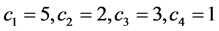 . The relative abundance of the subsets of species, taken separately, are:
 ,
,
 ,
,
 ,
,
 ,
,
 .
.
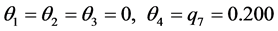
For the subset of species :
:
 ;
; 
For the subset of species 
 ;
; 
For the subset of species :
:
 ;
; 
For the subset of species :
:
 ;
; 
For the subset of species :
:
 ,
,
 ;
;
For the subset of species :
:
 ,
,
 ;
;
For the subset of species :
:
 ,
,
 ;
;
For the subset of species :
:
 ,
,

 ;
;
For the subset of species :
:
 ,
,
 ;
;
For the subset of species :
:
 ,
,
 ;
;
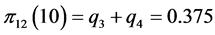
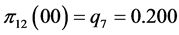
For the subset of species :
:
 ,
,
 ,
,  ,
,
 ,
,  ,
,
 ,
, .
.
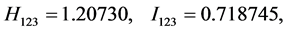
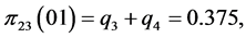
For the subset of species :
:
 ,
,
 ,
,  ,
,
 ,
,  ,
,
 ,
, .
.
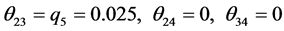
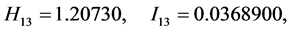
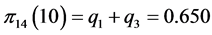
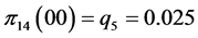
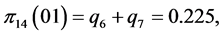
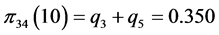
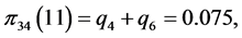
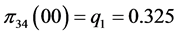
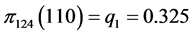
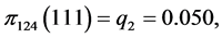
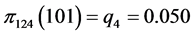
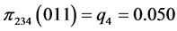
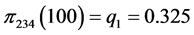
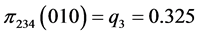
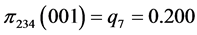
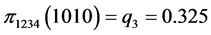
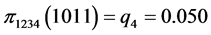
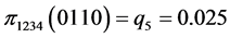
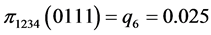
For the subset of species :
:
 ,
,  ,
,
 ,
,  ,
,
 ,
, .
.
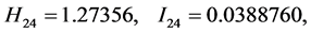
For the subset of species :
:
 ,
,
 ,
,  ,
,
 ,
,  ,
,
 ,
, .
.

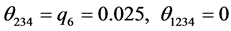
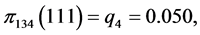
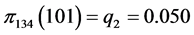
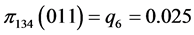
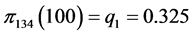
For the subset of species :
:
 ,
,
 ,
,  ,
,
 ,
,  ,
,
 (all the other patterns have a probability equal to 0)
Applying Formula (4), the weights are:
 ,
,  ,
,  ,
,
 ,
,  ,
,  ,
,
 ,
,  ,
,  ,
,
 ,
,  ,
, ,
,
 ,
, ,
, .
.
Applying Formula (3) with these weights, we obtain the amount of plant biodiversity on the island (at least as far as the four species, in this simplified example, are concerned), as measured by the weighted Gini-Simpson quadratic index: .
.
If the weights are ignored and we apply Formula (3) with all the weights equal to 1, we obtain the diversity on the island induced only by the abundance of the subsets of species, as measured by the classic Gini-Simpson index:![]() .
.
4. Conclusions
The classic Gini-Simpson index is the oldest and simplest measure of biodiversity. It takes into account only the relative abundance of the species from a habitat. As pointed out recently, this index of biodiversity does not behave well when the number of species is very large. The weighted Gini-Simpson index preserves the qualities of the classic index but behaves well when the number of species is very large. Moreover, the weights may be chosen in such a way that not only the relative abundance of species but also the number of species (richness), the distance between species, and the value of species are taken into account when the diversity in the habitat is measured. The weighted Gini-Simpson index continues to be a concave function of the relative abundance of species, allowing it to be used in the additive and multiplicative partitioning of diversity.
In the current applications of the weighted Gini-Simpson index the species are considered to be independent from the point of view of their individual relative abundance, which means that the joint relative proportion of a set of species is the product of the relative proportions of the species of this set. The first section of this paper summarizes the main variants of the weighted Gini-Simpson index recently introduced for dealing with such independent species. There are cases, however, when the species are not independent from the point of view of the relative abundance. The second section of this paper deals with interdependent species and the weighted Gini-Simpson index is adapted for dealing with such a more complex case. The new concept of distribution pattern variability of species is introduced, essentially based on Shannon’s entropy and Watanabe’s entropic measure of global interdependence. The new weighted Gini-Simpson index of biodiversity for interdependent species measures the amount of biodiversity induced by the abundance of species, the species richness, the value of species, and the distribution pattern variability of the subsets of interdependent species in the respective habitat.
The third section contains a numerical example which shows how the general formulas from the second section have to be applied.
References
- Gini, C. (1912) Variabilità e mutabilità. In: Pizetti, E. and Salvemini, T., Eds., Rome: Libreria Eredi Virgilio Veschi, Memorie di metodologica statistica.
- Simpson, E.H. (1949) Measurement of Diversity. Nature, 163, 688. http://dx.doi.org/10.1038/163688a0
- Jost, L. (2007) Partitioning Diversity into Independent Alpha and Beta Components. Ecology, 88, 2427-2439. http://dx.doi.org/10.1890/06-1736.1
- Jost, L. (2009) Mismeasuring Biological Diversity: Response to Hoffmann and Hoffmann. Ecological Economics, 68, 925-928. http://dx.doi.org/10.1016/j.ecolecon.2008.10.015
- Jost, L., DeVries, P., Walla, T., Greeney, H., Chao, A. and Ricotta, C. (2010) Partitioning Diversity for Conservation Analyses. Diversity and Distributions, 16, 65-76. http://dx.doi.org/10.1111/j.1472-4642.2009.00626.x
- Guiasu, R.C. and Guiasu, S. (2010) The Rich-Gini-Simpson Quadratic Index of Biodiversity. Natural Science, 2, 1130- 1137. http://dx.doi.org/10.4236/ns.2010.210140
- Guiasu, R.C. and Guiasu, S. (2003) Conditional and Weighted Measures of Ecological Diversity. International Journal of Uncertainty, Fuzziness and Knowledge-Based Systems, 11, 283-300.
- Lande, R. (1996) Statistics and Partitioning of Species Diversity and Similarity among Multiple Communities. Oikos, 76, 5-13. http://dx.doi.org/10.2307/3545743
- Guiasu, R.C. and Guiasu, S. (2010) New Measures for Comparing the Species Diversity Found in Two or More Habitats. International Journal of Uncertainty, Fuzziness and Knowledge-Based Systems, 18, 691-720.
- Whittaker, R.H. (1972) Evolution and Measurement of Species Diversity. Taxon, 21, 213-251. http://dx.doi.org/10.2307/1218190
- Whittaker, R.H. (1977) Evolution of Species Diversity in Land Communities. In: Hecht, M.K. and Steere, B.W.N.C., Eds., Evolutionary Biology, Plenum Press, New York, 1-67. http://dx.doi.org/10.1007/978-1-4615-6953-4_1
- MacArthur, R.H. (1965) Patterns of Species Diversity. Biological Review, 40, 510-533. http://dx.doi.org/10.1111/j.1469-185X.1965.tb00815.x
- MacArthur, R.H. and Wilson, E.O. (1967) The Theory of Island Biogeography. Princeton University Press, Princeton.
- Hill, M. (1973) Diversity and Evenness. A Unifying Notation and Its Consequences. Ecology, 88, 2427-2439.
- Rao, C.R. (1982) Diversity and Dissimilarity Coefficients: A Unified Approach. Theoretical Population Biology, 21, 24-43. http://dx.doi.org/10.1016/0040-5809(82)90004-1
- Pavoine, S., Ollier, S. and Pontier, D. (2005) Measuring Diversity from Dissimilarities with Rao’s Quadratic Entropy: Are Any Dissimilarities Suitable? Theoretical Population Biology, 67, 231-239. http://dx.doi.org/10.1016/j.tpb.2005.01.004
- Ricotta, C. (2005) Additive Partitioning of Rao’s Quadratic Diversity: A Hierarchical Approach. Ecological Modelling, 183, 365-371. http://dx.doi.org/10.1016/j.ecolmodel.2004.08.020
- Ricotta, C. and Szeidel, L. (2006) Towards a Unifying Approach to Diversity Measures: Bridging the Gap between the Shannon Entropy and Rao’s Quadratic Index. Theoretical Population Biology, 70, 237-243. http://dx.doi.org/10.1016/j.tpb.2006.06.003
- Hardy, O.J. and Senterre, B. (2007) Characterizing the Phylogenetic Structure of Communities by an Additive Partitioning of Phylogenetic Diversity. Journal of Ecology, 95, 493-506. http://dx.doi.org/10.1111/j.1365-2745.2007.01222.x
- Villéger, S. and Mouillot, D. (2008) Additive Partitioning of Diversity Including Species Differences: A Comment on Hardy and Senterre (2007). Journal of Ecology, 96, 845-848. http://dx.doi.org/10.1111/j.1365-2745.2007.01351.x
- Hardy, O.J. and Jost, L. (2008) Interpreting Measures of Community Phylogenetic Structuring. Journal of Ecology, 96, 849-852. http://dx.doi.org/10.1111/j.1365-2745.2008.01423.x
- Ricotta, C. and Szeidel, L. (2009) Diversity Partitioning of Rao’s Quadratic Entropy. Theoretical Population Biology, 76, 299-302. http://dx.doi.org/10.1016/j.tpb.2009.10.001
- Sherwin, W.B. (2010) Entropy and Information Approaches to Genetic Diversity and Its Expression: Genomic Geography. Entropy, 12, 1765-1798. http://dx.doi.org/10.3390/e12071765
- De Bello, F., Lavergne, S., Meynard, C.N., Lepš, J. and Thuiller, W. (2010) The Partitioning of Diversity: Showing Theseus a Way out of the Labyrinth. Journal of Vegetation Science, 21, 992-1000. http://dx.doi.org/10.1111/j.1654-1103.2010.01195.x
- Tuomisto, H. (2010) A Diversity of Beta Diversities: Straightening up a Concept Gone Awry. Part 1. Defining Beta Diversity as a Function of Alpha and Gamma Diversity. Ecography, 33, 2-22. http://dx.doi.org/10.1111/j.1600-0587.2009.05880.x
- Tuomisto, H. (2010) A Diversity of Beta Diversities: Straightening up a Concept Gone Awry. Part 2. Quantifying Beta Diversity and Related Phenomena. Ecography, 33, 23-45. http://dx.doi.org/10.1111/j.1600-0587.2009.06148.x
- Guiasu, R.C. and Guiasu, S. (2011) The Weighted Quadratic Index of Biodiversity for Pairs of Species: A Generalization of Rao’s Index. Natural Science, 3, 795-801. http://dx.doi.org/10.4236/ns.2011.39104
- Guiasu, R.C. and Guiasu, S. (2012) The Weighted Gini-Simpson Index: Revitalizing an Old Index of Biodiversity. International Journal of Ecology, 2012, 10 p.
- Crooks, K.R. and Soulé, M.E. (1999) Mesopredator Release and Avifaunal Extinctions in a Fragmented System. Nature, 400, 563-566. http://dx.doi.org/10.1038/23028
- Shannon, C.E. (1948) A Mathematical Theory of Communication. Bell System Technical Journal, 27, 379-423, 623-656. http://dx.doi.org/10.1002/j.1538-7305.1948.tb01338.x
- Watanabe, S. (1969) Knowing and Guessing. Wiley, New York.
- Guiasu, S. (1977) Information Theory with Applications. McGraw-Hill, New York.