Natural Science
Vol.6 No.4(2014), Article ID:43342,20 pages DOI:10.4236/ns.2014.64020
Gravitational transformation of gaseous clouds: The formation of spiral galaxies and disk planets
![]()
Orvokkikatu 8, Naantali, Finland; ap315@cam.ac.uk, andrei.pavlov1@gmail.com
Copyright © 2014 Andrei Pavlov. This is an open access article distributed under the Creative Commons Attribution License, which permits unrestricted use, distribution, and reproduction in any medium, provided the original work is properly cited. In accordance of the Creative Commons Attribution License all Copyrights © 2014 are reserved for SCIRP and the owner of the intellectual property Andrei Pavlov. All Copyright © 2014 are guarded by law and by SCIRP as a guardian.
Received 4 December 2013; revised 4 January 2014; accepted 11 January 2014
Keywords:Gravitation; Planets; Saturn’s Rings; Computer Simulation; Planet’s Interior Structure; Formation of Galaxies; Spiral Galaxies; N-Body Simulations
ABSTRACT
Gravitation is one of the central forces playing an important role in formation of natural systems like galaxies and planets. Gravitational forces between particles of a gaseous cloud transform the cloud into spherical shells and disks of higher density during gravitational contraction. The density can reach that of a solid body. The theoretical model was tested to model the formation of a spiral galaxy and Saturn. The formations of a spiral galaxy and Saturn and its disk are simulated using a novel N-body self-gravitational model. It is demonstrated that the formation of the spirals of the galaxy and disk of the planet is the result of gravitational contraction of a slowly rotated particle cloud that has a shape of slightly deformed sphere for Saturn and ellipsoid for the spiral galaxy. For Saturn, the sphere was flattened by a coefficient of 0.8 along the axis of rotation. During the gravitational contraction, the major part of the cloud transformed into a planet and a minor part transformed into a disk. The thin structured disk is a result of the electromagnetic interaction in which the magnetic forces acting on charged particles of the cloud originate from the core of the planet.
1. INTRODUCTION
We simulate the formation of spiral galaxies and disk planets and their inner structures using a novel N-body model. Particularly, the ringed planets are especially interesting. In our numerical approach, the dynamics of selfgravitating N-body systems is considered using Newtonian gravitational interaction [1], conservation of angular momentum by applying Kepler’s second law [2] to N bodies and thermodynamic adiabatic law. In addition, the electromagnetic interaction is included in the formation of the structured disk of Saturn. The dynamics of Saturn and its rings is investigated in detail [3]. We assume that both the planet and its disk are formed simultaneously during gravitational contraction of a large cloud of particles. The initial rotation of the system is included because the result of the gravitational contraction is a rotating system. At initial time, the particles are randomly distributed within the deformed sphere and all particles of the n-body system have equal angular velocities. Although Jeans condition of the hydro dynamical equilibrium predicts instability for light systems such as Saturn [4], the initial state of the cloud may exist when applying a different approach. The Jeans condition deals with average density and pressure to characterize the hydro dynamical equilibrium state of the system. It is supposed that the particles are localized in different smaller clouds having sizes much smaller than the distances between them. Then the density can be described by 3N d-functions. In this case, the temperature of each body is differrent from the temperature of the whole system. One can substitute the Jeans mass for that of Saturn and calculate an effective temperature of the system of Teff = 570 K using the initial radius 1 × 10⁹ m and the mass of a proton. The corresponding velocity of a proton is about 4000 m/sec. One can suppose that the local clouds are expanding while the whole system is contracting. The temperature of the local cloud will decrease and proton’s velocity will decrease as well. The contraction time obtained from the simulation is of the order of 1 × 10⁵ sec. During this time, if the proton moves with average velocity of 1000 m/sec., it will travel the distance of 1 × 10⁸ m that is about one tenth of the initial radius of the N-body sphere. Due to random directions of local thermal movement, not many protons escape from the system.
This assumption allows considering systems much lighter than the Sun. It is supposed that the ith body of the N-body cloud had a mass mi and coordinated xi, yi, zi. Then the total mass is given by
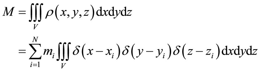 (1)
(1)
Although one can associate the mass M with the average density M = ravV, this density used in the Jeans condition is different from the density obtained in the present model
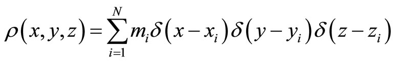 . (2)
. (2)
The stability of the system is revealed during the simulation when the relative positions between the bodies change very slowly at the beginning of the process during almost one third of the contraction time.
A new simulation program is designed for the modeling of the gravitational contraction of the self-gravitating N-body system. The system has a shape of the sphere slightly flattened along the axis of rotation. Because the mass of the cloud is given by 3N d-functions, the traditional codes are difficult to apply to this system. We use a direct implementation of equations of motion combining two mechanisms: the Newtonian gravitational interaction and conservation of angular momentum. The algorithm is based on calculations of the gravitational accelerations of all bodies and their displacements using the gravitational law in its original differential form
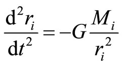 . In calculations of the gravitational masses, positions of all bodies are used. The rotational velocities wi are obtained by applying the Kepler’s second law for small angles given by
 . During gravitational attraction, the velocities of the bodies increase towards the center of mass. The total velocity of each body is a vectorial sum of the radial and tangential (orbital) velocities. An increase of the radial velocity results in an increase of the angular velocity calculated from the Kepler’s formula. As a result, the remote particles will rotate slower than those situated closer to the center. Due to non-spherical geometry of the cloud, the disk will develop at the edges of the cloud in the rotation plane. In addition, rotational movement of the system will lead to its shrinking along z-axis and flattening of the planet. The charged particles of the faster rotating core of the planet will establish the magnetic field. This magnetic field will interact with the charged particles of the disk and, finally, this interaction results in formation of Saturn’s structured disk.
2. THEORETICAL
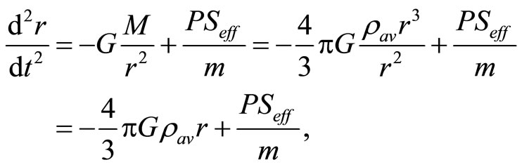
It is assumed that prior to its present form the Saturnlike planet had consisted of a slightly deformed spherical cloud of particles. The number of particles in gravitational systems may be very large and ill-defined and, therefore, to simplify the model we combine neighboring particles into clusters and consider the gravitational interaction between these clusters resulting in self-contraction of the cloud. One can imagine that two particles situated near to each other will have the same gravitational aceleration due to interaction with all the other particles. Therefore, by combining them into cluster means that we consider the movement of their center of mass. The gravitational law for a cluster can be written in the form
 (3)
(3)
where G is the universal gravitational constant , M the gravitational mass, rav an average density, r the relative position between the cluster and the center of mass of the whole system, P is the internal pressure, Seff an effective cross section and m the mass of the cluster. The initial condition comprises randomly distributed positions, r, of the clusters. Their speeds are zero and the average density rav(t = 0) = r0. Suppose that the time steps are small enough so that during one time step the average density does not change. Then the solution of the differential Eq.3 is given by
 . (4)
. (4)
At the beginning of the process the cloud contracts without changing its structure. Suppose that the internal pressure is very small at the beginning of the process. Then Eq.3 is a simple harmonic oscillator with the frequency given by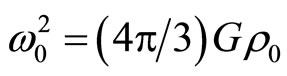 . The speed
 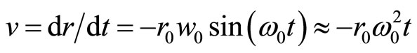 for
for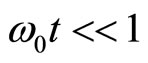 , being a linear function of r at a particular time. At small internal pressure the average density rav is given by
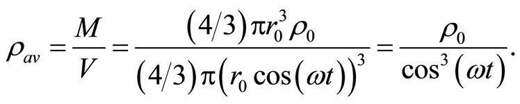 (5)
(5)
This density does not depend on the position, r, and is therefore constant within the volume of the cloud.
Consider Eq.3 when speeds are not zero. By substituting r = Acos(wt) + Bsin(wt)+ pressure term into Eq.3 we get the solution at A = r1, B = –v1/w and w2 = 4p/3Grav, here r1 and v1 are position and the speed of the cluster at time t1. The following phenomenon can be deduced from this result: Consider any two clusters labelled i and j situated close to each other. Then there may exist a time d tij after which their positions from the center become equal i.e.
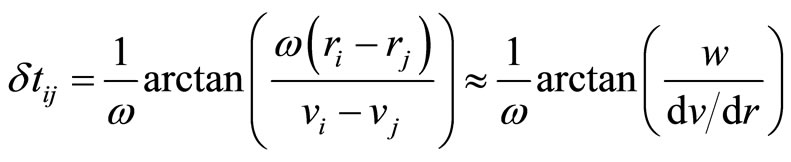 . (6)
. (6)
dtij depends on neither r1 nor r2 , but only on the derivative dv/dr. This means that more than two clusters can reach the same radius and this process will take place in a whole volume resulting in increasing density at places in which dv/dr satisfies the equation
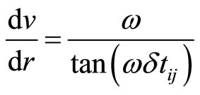 . (7)
. (7)
Then the local density will vary leading to formation of structured spherical layers in accordance with the equation
 , (8)
, (8)
where v is the speed and r the position of the layer from the center of mass. One can expect that the amplitude of the oscillation of the local density would increase towards the center of mass because there are fewer clusters there and their speeds are smaller.
The rotational movement is described using Kepler’s second law. Due to small time intervals after which all velocities are recalculated, the Kepler’s law can be applied to small angles
 , (9)
, (9)
where wi1 and wi2 are rotational velocities separated by one time step. The associated additional displacement is calculated adding to a full displacement of the cluster.
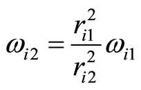
There arises a question how angular momenta of the clusters relate to each other? One can expect that clusters situated closer to the center of mass will have different angular velocities due to strong dissipation process. For remote clusters, the gravitational masses will differ very little because most of the clusters are concentrated closer to the center. Therefore, for a remote cluster one can rewrite Eq.9 using Eq.4 as
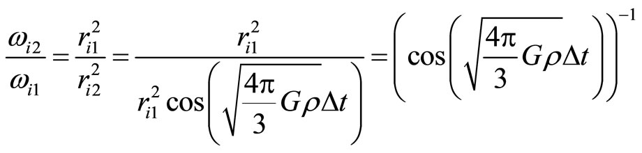 . (10)
where Dt is the travelling time from ri1 to ri2. This ratio does not depend on ri. For the same travelling times other remote clusters will have the same relation leading us to a conclusion that
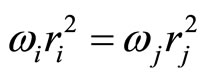 . (11)
The meaning of this equation is that during the gravitational contraction the angular momenta of the remote clusters equalize. Then there exists a curve w(r) which fit all the values wi(ri) of remote clusters. One can expect that this curve terminates on the surface of the planet. Then Eq.11 can be written as
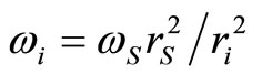 , (12)
here rs is the planet’s radius and wS its angular velocity. These parameters are known for Saturn and, therefore, this equation can be used to get angular velocities of the remote clusters during planet’s formation. We would notice that the final angular velocities will change dramatically from Eq.12 due to the electromagnetic interaction mechanism described below. In addition to gravitational contraction of the cloud, the disk itself shrinks along the z-axis. This gravitational shrinking is almost uniform resulting in a very thin disk. First estimations of the vertical thickness of the disk based on the photometric measurements yielded a thickness of one km [5,6]. Then photo-polarimeter experiments revealed that the thickness is 200 m [7]. The effective thickness now is estimated to be of the order of few tens of meters reported by Rosen and Lissauer [8], Chakrabarti [9] and Rosen et al. [10].
The magnetic forces play a very important role in creation of the structured disk. This mechanism takes place at final stage of the planet’s formation. The magnetic field is established by the rotating planet’s core. In the equatorial plane, the plane of the disk, the angle between the velocity vector and magnetic field is p/2 and therefore the magnetic force will be given simply by Fm = qvB where q is the charge of a particle. The additional increase of the orbital velocity is given by
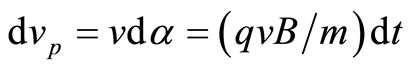 , (13)
where a is a turning angle. The magnetic field needed for turning the particle onto the orbit, corresponding to the angle alpha of p/2, is obtained from Eq.13
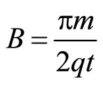 . (14)
It is remarkable that the magnetic field does not depend on the velocity. It means that all similar charged particles of equal masses situated at the same position from the center will turn on their orbits during the same time. A typical gravitational contraction time of the final stage when the system is already separated into two subsystems, planet and disk-forming cloud, is about 10,000 seconds. One can estimate values of the magnetic field needed to turn particles on to their orbits. For electron the magnetic field is 0.9 × 10⁻¹⁵ T. For ionized hydrogen atom it will be 1.5 × 10⁻¹² T. How many charged particles have to rotate to produce that magnetic field? To simplify the problem, consider only one circular loop of radius R inside the planet. Then the magnetic field B outside the planet at equatorial plane is given by
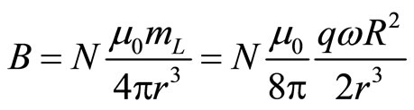 , (15)
where mL is the magnetic dipole moment, r is the position from the center, q is the charge of a particle, N number of the particles and m0 permeability of free space m0 = 4p × 107 Henry/m. For an orbit of radius R = 2 × 10⁷ m, the angular velocity estimated from Eq.12 w =1 × 10⁻³ rad/sec. Using the value of elementary charge q = 1.6 × 10⁻¹⁹ C, the magnetic field B = 1 × 10⁻¹⁰ T and mass of hydrogen atom mH = 1.66 × 10⁻²⁷ kg, the calculated number N is 2 × 1029 and the total mass of N particles is as small as around 300 kg. This estimation suggests that during the gravitational contraction, a slow rotation of a large number of charged particles produces a sufficient magnetic field to enable formation of the disk. Probably, the magnetic field at that stage is much stronger.
One can conclude that electrons will form a ring at earlier times and much further from the planet than hydrogen atoms. The electron’s belt should rotate in opposite direction to the main disk. The ring’s structure observed on Saturn’s disk can be related with different atomic structure. The magnetic force results in separate different rings associated with different masses of the particles and different positions at the time when the magnetic field “switched on”. The disk is decomposed into light and heavy elements during electro-magnetic interaction. The heavier particles will establish rings closer to the planet. Very heavy particles will be not affected by the magnetic field. Therefore, these particles will continue their movement towards the planet remaining spokes-like structures on the disk. When approaching the planet the particles interact with each other and the effective cross section increases resulting in widening the spokes towards the planet’s surface. This is clearly seen in the images of the B-ring. The gaps between the rings indicate the differences in the atomic masses. This can be possible if chemical composition of the particles is simple and particles consist of few atoms. The mass of the disk, in accordance with this mechanism, is much smaller than the mass of the planet. This correlates well with the observational data. The elliptical orbits observed on the disk support this model because the elliptical orbits may originate only if the particles change their trajectories from free fall.
To estimate the temperature of the system we consider each cluster as a volume of particles and correlate the thermal energy with the distribution of the kinetic energy of the system [11]. The classical methods for calculating the temperature could not be used directly because most of them describe systems in equilibrium at a constant temperature and constant chemical potential. However, we suppose that for a short period of time during which the acceleration is constant, the chemical potential is constant for a thin spherical layer. Therefore, the whole spherical volume can be divided into thin layers and we calculate the temperature of each layer from the equation
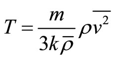 , (16)
where m is the mass of a particle,  is the average density, r is the local density,
  is the average squared velocity of the layer.
To estimate the internal pressure and its influence on the disk structure one can write an equation for the work of the force FP associated with the pressure acting on a particle. The work of this force will be equal to the change of the kinetic energy of the particle.
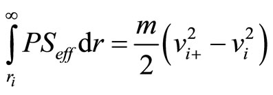 , (17)
where Seff is a cross section of the particle, vi+ the velocity of the particle at position ri without pressure and vi the velocity of the particle at the same position under pressure. The adiabatic process is described by the equation 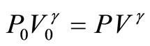 or
or
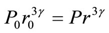 . (18)
The values P0, V0 and r0 will be referred to the planet’s surface. Suppose that at a position rA the pressure and gravitation compensate each other. Then
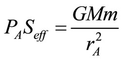 , (19)
being M a mass of the planet and m particle mass. Then using Eqs.18 and 19 the surface pressure can be written as
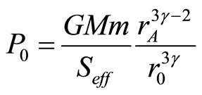 . (20)
The integral Eq.17 can be transformed as follows
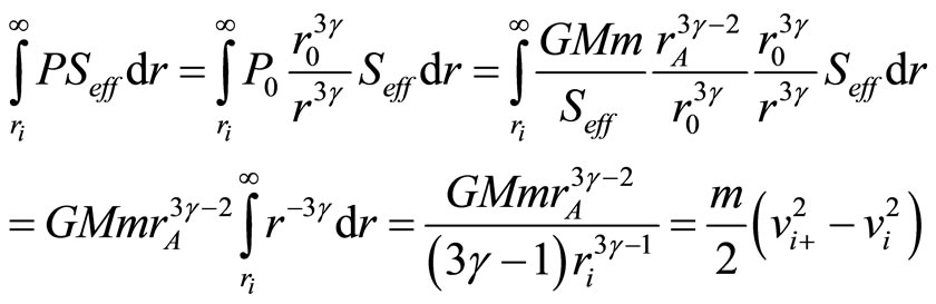 (21)
(21)
Then the actual velocity vi is given
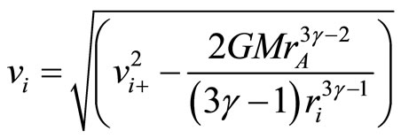 . (22)
The velocity at the equilibrium state
 (23)
(23)
The value of g is calculated using a well-known relation g = CP/CV. One can expect complex molecular structures with a big effective number of degrees of freedom including vibration. Then a model of the bent triatomic molecule can be applied. For this molecule type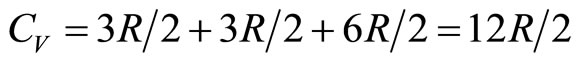 ; CP = 14R/2; g = 7/6. Some examples of this type of molecules are H2O, ozone O3, SO2, H2S etc. If the number of degrees of freedom is very large or infinite then
 (24)
(24)
If there are different types of particles then the different positions are obtained using the condition Eq.20
 (25)
(25)
This equation implies the formation of structured disk. The radius depends on both parameters particle mass mi and its effective cross section Seff i. During the formation of the planet the adiabatic coefficient g can change also starting form 1.7 for one-atom particles down to 1 for many atom particles. The structure of the disk associated with the variation of g depends on the number of degrees of freedom. Then using g =L1/L2 where L1 and L2 are integers one can write Eq.25 as
 (26)
(26)
This equation explains the formation of numerous ringlets in the disk of Saturn due to variations of L1 and L2. Because these values are integers, the discrete structure is obtained. Comparison of the contributions of the gravitational attraction force and the force associated with the pressure reveals dramatic decrease of the pressure at large positions due to its dependence Fpµ r–3g whiles the gravitational force F µ r–2.
3. COMPUTER SIMULATION
A special N-body simulation computer program has been designed for continuous calculation of the position, speed and acceleration of each cluster during gravitational contraction. The particles are randomly distributed within a deformed spherical volume at the initial time. The deformed shape is obtained by flattening the sphere by a coefficient 0.8 along z-axis, the axis of rotation.
The whole time range consists of short periods. During each period of time the clusters have constant accelerations that are different for different clusters. At the end of each period the acceleration of every cluster is re-calculated taking into account the new positions of the other clusters. In addition, rotational velocities are calculated using Eq.9 and its contribution is added into final displacements. In this model we use hydrogen atoms because it is believed that Saturn consists mostly of hydrogen. The total number of clusters used is 2500, having equal masses. These clusters have a total mass of 5.68 × 1026 kg that is the round mass of Saturn.
The process of gravitational contraction can be divided in three stages.
1) The First stage is the gravitational contraction of the slowly rotating slightly flattened large spherical cloud. This process takes about two thirds of the total contraction time from the beginning during approximately 1 × 10⁵ seconds. The cloud decreases in size without significant change of its geometry. The dynamics of the cloud at this stage are revealed in Figure 1. The cloud is shown in two planes, the xy plane of rotation, and the xz plane.
2) During second stage the cloud separates into the planet’s cloud and the disk. During this stage the structure of the cloud changes and the disk starts to form. The second stage is lasting from 1 × 10⁵ to 1.45 × 10⁵ seconds demonstrated in Figure 2. The gravitational contraction of the central part of the cloud occurs faster than the contraction of the disk.
3) Figure 3 shows third stage that is a shortest one during 1.45 × 10⁵ to 1.5 × 10⁵ seconds. At this stage, the planet approaches its present geometry and dynamics. The disk has still a relatively large mass of the order of 1 × 1024 kg and contracts as well. But, the processes in the planet’s cloud occur much faster than the contraction of the disk. The magnetic field is established from the rotating core of the planet. The radiation coming from the planet ionizes atoms in the disk’s cloud. The magnetic forces acting on charged particles turn the particles onto round orbits. The difference in masses and charges of different ionized particles will result in formation of structured rings. Heavy particles continue their movement further towards the planet remaining traces on the disk known as spokes. The mass of the disk decreases dramatically because heavy particles move towards the planet. The stripes on the surface of the planet may be
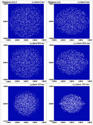
Figure 1. The development of the N-body system is shown for first stage of the formation from the beginning of the contraction during two thirds of the contraction time. The graphs are shown in two planes, the xy plane of rotation, graphs on the left, and in xz plane, graphs on the right. The corresponding times are (a) 0 sec., (b) 5.0 × 10⁴ sec. and (c) 1.0 × 10⁵ sec. The cloud contracts without significant change of its structure. The disk just starts to appear at the end of this stage.
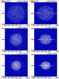
Figure 2. The continuation of the formation process started in Figure 1 is shown for the second stage. The cloud separates into the central spherical cloud and the disk. The disk is relatively thick and massive. The system is shown for the times of (a) 1.20 × 10⁵ sec., (b) 1.34 × 10⁵ sec. and (c) 1.40 × 10⁵ sec.
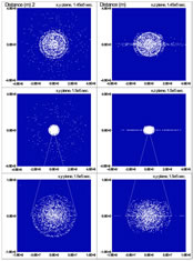
Figure 3. The most dynamical final phase of the formation of the planet and its disk is shown. The planet contracts much faster than the disk resulting in formation of the planet. The disk contracts slower and its diameter decreases slightly. The magnetic field is established and charged particles turn to their round orbits due to magnetic forces. Heavy particles continue their movement towards the planet leaving spokes-like structure on the disk. Approaching the surface of the planet these heavy particles remain stripes on the surface indicating this stage of the planet formation. The gap between the planet and the disk is seen where the internal pressure dominates the gravitation. The planet and its disk is shown for the times of (a) 1.45 × 10⁵ sec., (b) 1.50 × 10⁵ sec. The graphs (c) are enlargement of central part of the graphs (b).
associated with this process as well. Finally, the disk becomes thinner and lighter. There is a region of very low density between the planet and the disk where the internal pressure dominates the gravitation. Comparison of the velocities of the simulation and observed orbital velocities of the disk reveal a perfect correlation. The compared values are collected in Table 1. The observed data about Saturn’s disk are reported by Cuzzi et al. [12], Esposito et al. [13] and by Nicholson et al. [14]. The velocity difference associated with the radiation coming from the planet decreasing the velocities of the clusters in accordance with Eq.23 is around 25%.
The inner structure of the planet is a complex composition of spherical shells separated by regions of very low density. Figures 4 and 5 reveal how randomly distributed clusters combine into spherical shells during gravitational contraction. The outer shell of Saturn has a spherical shape but is open at the top and bottom. The equatorial radius is about 6 × 10⁷ m and that along the z-axis 5 × 10⁷ m. This agrees very well with the observed values. At final stage, around 5000 seconds, the dynamics of the formation process is most dramatic. The central region of the planet is almost empty at 1.45 × 10⁵ seconds and during the last 5000 seconds it became filled with very fast moving bodies. Some of the bodies go through the center of mass of the planet and move away. Most of them will be trapped in the outer shells but some of them can escape from the planet through the equatorial strip and form the orbiting satellites. Therefore, the information about Saturn’s satellites may reveal the information about the inner structure of the planet.
The surface of the planet is very rough, hundreds of km in height variations. The relief of the planet changes dramatically from middle altitudes to the equator. At the equatorial strip the height variations are as large as 4000 km and there are pillar-like structures of enormous height here. The width of this strip is around 12000 km.
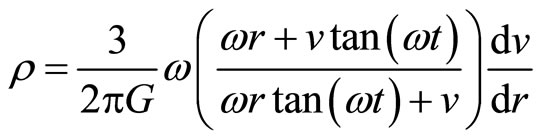
The time development of the density of the planet is plotted in Figures 6-8. The initial density is very low, about 0.5 kg/m3. It starts to grow during gravitational contraction and a number of peaks can be seen after 1 × 10⁵ seconds corresponding to appearing of spherical shells. The density at peaks grows significantly to few thousands of kg/m3 at final stage and varies between 1000 kg/m3 and 4000 kg/m3 and increases towards the center of the planet reaching almost 4 × 10⁴ kg/m3 at around 1.0 × 10⁷ m from the center. The density of the outer shell is around 3000 kg/m3. This suggests that the surface of Saturn is a solid-state material. However, the central region of the planet has a very low density. There are also regions of very low density between the shells. There is a post-formation process. This is a long-term process of electro-magnetic interaction between charged particles. The electrostatic interaction between positively charged particles and electrons may result in neutralization of the particles.
The dynamics of the formation process can be seen in Figures 9 and 10 where velocities of all clusters versus position are shown for different times. The observed orbital velocities of Saturn’s rings and satellites are also included combined in Table 1. The velocities of the simulated disk have a perfect correlation with the observed data. The result of the simulation reveals the escape velocity at the Saturn’s surface of 3.2 × 10⁴ m/sec after 1.5 × 10⁵ seconds that is very close to the observed value of 3.5 × 10⁴ m/sec. The small difference is present because some of the clusters of the disk did not approach the planet yet. When those clusters fall onto the planet the mass of the planet increases and the escape velocity increases a little as well. In Figure 10 both velocities, without influence of the pressure and under pressure, are shown. The model of bent triatomic molecule is used for which g = 7/6. The last graph demonstrates a perfect match of the simulated and measured values. The impact of the internal pressure results in the much lower density inside a big gap between the planet’s surface and the inner edge of the B-ring. However, heavy particles having small effective cross section exist inside this gap.
It is interesting that during the final stage, around 5000 seconds, of the gravitational contraction the central region of the planet is filled with bodies whose velocities vary from near to zero up to 25 km/s. The bodies have a high density and their velocities are enough to escape from the planet. There are natural obstacles for them, the outer shells. During this escape the bodies can be trapped within the shells but some of them can go through. Those bodies that came through the shells became the Saturn’s satellites. This also explains why the satellites are different in chemical composition, density etc. They initially formed in different shells inside Saturn. Therefore, the knowledge about the satellites may help to understand the atomic structure of the interior shells of Saturn.
The rotational dynamics is presented in Figure 11. Angular velocities of the clusters versus position are plotted for different times. The solid line is calculated form Eq.12 using the measured Saturn’s period of rotation of 10.233 hours. The surface of Saturn is also marked in the graph. Although at the beginning of the contraction all the clusters have the same angular velocity of 1.5 × 10⁻⁷ rad/s, the clusters of the disk approach the curve given by Eq.12 during the gravitational attraction, revealing the equalizing of their angular momenta. The clusters of the planet’s cloud situated closer to the center have a variety of angular velocities revealing a strong dissipation of the kinetic energy and a rise of the temperature.
For the calculation of the temperature each cluster is considered as a volume of separate atoms. The process of
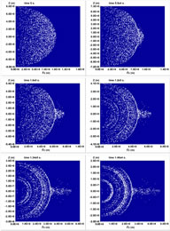
Figure 4. The formation of the inner structure of the planet is shown in cylindrical coordinates, z and rz, for the period from the b ginning up to 1.4E4 seconds of the contraction process.
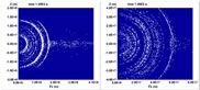
Figure 5. The final stage of the formation of the inner structure of Saturn is shown in cylindrical coordinates, z and rz for 1.45 × 10⁵ s and 1.50 × 10⁵ s.

Table 1. The observed orbital velocities and positions reported by NASA using the data of Voyager mission of a few Saturn’s rings and satellites and the data obtained from computer simulation reported in this paper. The observed data are indicated in Figures 3 and 4. The results of simulation correspond to the graph (c) of Figure 5.
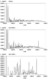
Figure 6. The local density of the cloud vs. position from the center is shown for 0, 5.0 × 10⁴ s and 1.2 × 10⁵ s.
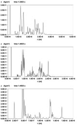
Figure 7. The local density of the cloud vs. position from the center is shown for 1.34 × 10⁵ s, 1.40 × 10⁵ s and 1.45 × 10⁵ s.
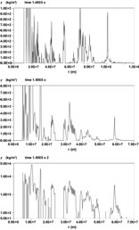
Figure 8. The local density of the cloud vs. position from the center is shown for 1.048 × 10⁵ s and 1.50 × 10⁵ s.
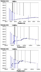
Figure 9. Velocities of the clusters during the first and second stages corresponding to Figures 1 and 2 versus position are shown. The Saturn’s few rings and satellites are indicated using data of Table 1. The symbols associated with the rings are provided with the vertical lines connected to x-axis downwards whereas satellites have lines connected to the top frame of the graph. The velocities are shown for the times (a) 1.00 × 10⁵ s, (b) 1.34 × 10⁵ s and (c) 1.40 × 10⁵ s.
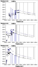
Figure 10. Velocities of the clusters during final stage corresponding to Figure 3 versus position are shown. The Saturn’s few rings and satellites are indicated. The rings are associated with the vertical lines connected to x-axis downwards whereas satellites have lines connected to the top frame of the graph. The velocities are shown for the times (a) 1.45 × 10⁵ sec., (b) 1.48 × 10⁵ sec. and (c) 1.50 × 10⁵ sec. Both velocities are shown, without influence of the pressure (upper symbols) and when the system is under pressure. The gap is revealed in the final graph stretched from the surface of the planet to the inner edge of the B-ring.
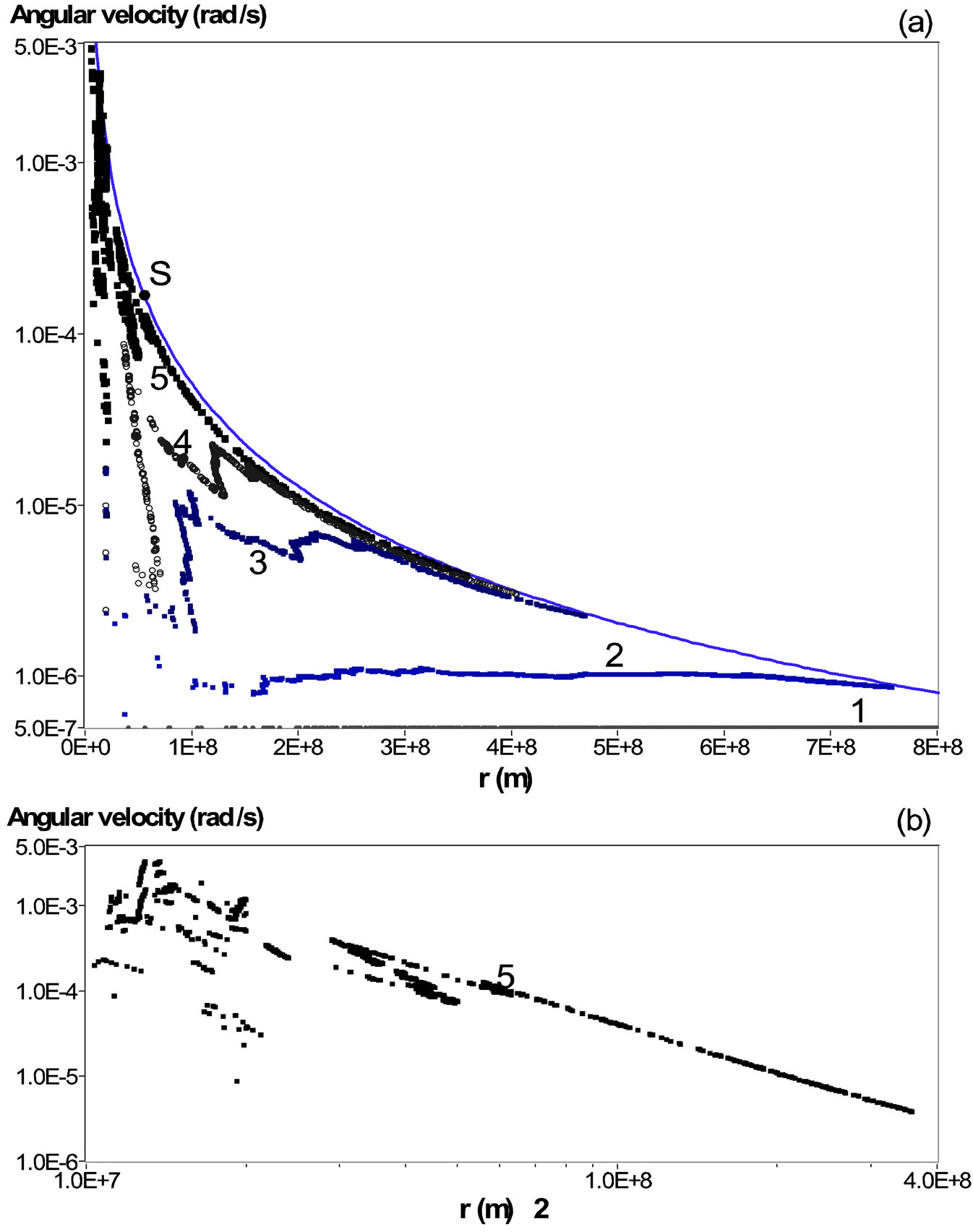
Figure 11. Kepler’s angular velocities of the clusters versus position are shown for different times of the formation process shown in Figures 1-3. At initial time, all the clusters have equal angular velocities of 5.0 × 10⁻⁷ rad/sec. (symbols 1). The results of simulation are shown for the times of 1.0 × 10⁵ sec. (squared symbols 2), 1.34 × 10⁵ sec. (squared symbols 3), 1.45 × 10⁵ sec. (round symbols 4) and 1.50 × 10⁵ sec. (squared symbols 5). The surface of Saturn is indicated with solid round symbol S. The solid line is calculated using Eq.12. The inset graph shows the angular velocities of the clusters 5 where both position and angular velocity are shown in logarithmical scale revealing a perfect straight line.
the gravitational contraction is an adiabatic one. The temperature of the contracting cloud is calculated using Eq.16 and the results are shown in Figure 12. The temperature has few prominent maxima. During the contraction process the temperature is higher at the edges of the cloud and then reaches its maximum of about 1 × 10⁶ K in the central region of the planet at final stage.
For simulation of formation of a spiral galaxy, we assume that initially the elliptical E-type shape of the galaxy is obtained by proportional shrinking the spheroid along yand z-axes by 0.8, the most frequently observed apparent axis ratio [15-18]. Initially the particles are randomly distributed within this volume. The radial velocities of all particles are zero. The galaxy has slow rotation on z-axis. The number of the particles in the galaxy N = 2000. In addition, 300 particles are created outside the body of the galaxy to study the dynamics of the process in more detail. The galaxy has the total mass of 1 × 1043 kg, a typical galaxy’s mass. The particles have equal masses m = 5 × 1039 kg. The starting angular velocity was of the order of 1 × 10–15 rad/s and the corresponding initial period of rotation T = 2p/w was about
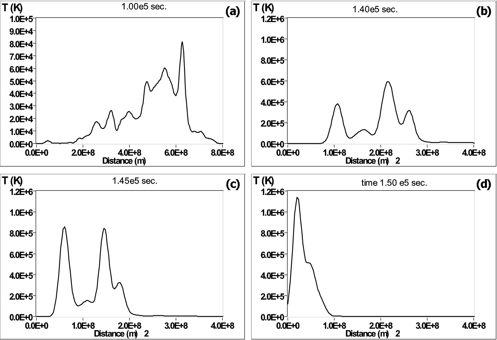
Figure 12. The temperature of the cloud calculated during simulation process by using Eq.16 is shown for different times (a) 1.00 × 10⁵ sec., (b) 1.40 × 10⁵ sec., (c) 1.45 × 10⁵ sec. and (d) 1.50 × 10⁵ sec.
two hundred million years.
Figure 13 demonstrates the time evolution of the Etype elliptical galaxy and its transformation to Seyfert Sc-type galaxy. The initial radius along x-axis is 750 kpc. The galaxy rotates anticlockwise in xy-plane. The time of formation of the spiral is about 4 × 10¹⁵ seconds which is a little smaller than the initial period of rotation. The formation of the spiral can be divided in three stages. The first stage lasts from the beginning of the contraction until the formation of two different geometrical shapes, the central part and two regions apart of it, after 3.35 × 10¹⁵ sec. (Figure 13(d)). The central part of the galaxy becomes more spherical, this is the future core of the spiral. The particles outside this region becomes more flattened and concentrated inside two symmetrical regions opposite to each other. These will form the two arms of the spiral. The second stage is further development of the core structure and the two arms. It lasts between 3.35 × 10¹⁵ sec. and 3.90 × 10¹⁵. At the end of this stage the spiral is formed (Figure 13(f)). During the last stage, the further evolution of the galaxy can be considered as the contraction of two different systems, the core and the two arms. The core of the galaxy rotates and contracts much faster than the arms. During this stage most dynamics occurs in the core, and the arms of the spiral get only minor changes.
The comparison of the photo images of these type spiral galaxies such as NGC 2997, NGC 157, NGC1566, NGC 300 and others, reveals an excellent similarity of the shape of the arms and the core shown in Figure 14. One can conclude that almost any shape of a galaxy will transform into spheroid and surrounding it spiral arms and disks are a reminder of this transformation. This is in accordance with the hypothesis that most of stellar systems are triaxial [19].
4. CONCLUSIONS
The formation of a spiral galaxy, Saturn, its disk and interior, along with dynamical properties is simulated using a novel gravitational N-body model for system of particles and the computer simulation program developed by the author. The self-gravitating cloud of particles contracts in accordance with Newtonian mechanics where interaction between all particles is considered. Particularly, the model considers an extremely large number of particles comprising the gaseous cloud. The rotation of the cloud is described by Kepler’s second law applied to a short periods of time as a result of the conservation of angular momentum. The simulation results show that gravitational contraction produces complex structures inside planets and stars. For disk planets like Saturn, the model predicts the formation of structured disk. Both disk and interior are complex structures. The formation of the structured disk is incorporated with the interaction between the magnetic field and the charged
Figure 13. The time evolution of the E-type elliptical galaxy and its transformation to Seyfert Sc-type spiral. The galaxy rotates anticlockwise. The turning angle is indicated in Figures 1(a)-(e). After 3.7 × 10¹⁵ seconds of the gravitational contraction, the core of the galaxy rotates more than 10 times faster than the arms.
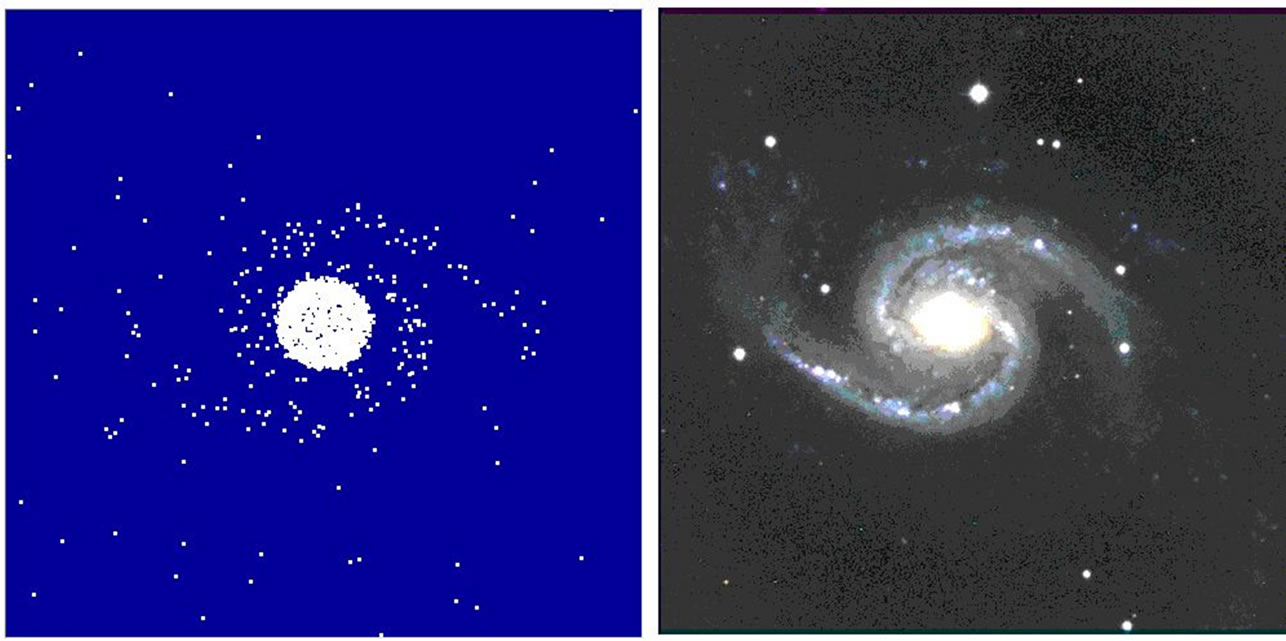
Figure 14. Comparison of the simulated galaxy and NGC1566. The plain of rotation of the simulated galaxy is tilted at 22 degrees relative to the plain of the picture.
particles. The planet consists of several spherical shells having high density and the outer shell has the density of a solid-state material.
The theoretical model and computer simulation predict the shape of spirals of the spiral galaxies. The dynamics of rotating elliptical galaxy and its transformation to a Seyfert spiral galaxy is modeled. The two arms and core of the spiral are the result of the gravitational interaction and differential rotation. The results of the simulation show that the type of the spiral galaxy is determined mainly by the initial shape of the galaxy and its initial rotation. The computer simulation reveals that a spiral shaped galaxy is a result of the transformation of a cluster of non-spherical symmetry. In addition, the spiral can form if the contraction time is larger than the period of rotation of the galaxy.
REFERENCES
- Newton I. (1687) Philosophiae naturalis principia mathematica (Mathematical principles of natural philosophy).
- Kepler J. (1619) De harmonice monde (The harmony of the world).
- Cuzzi, J.N., Lissauer, J.J., Esposito, L.W., Holberg, J.B., Marouf, E.A., Tyler, G.L. and Bouschot, A. (1984) Saturn’s rings: Properties and processes. In: Greenberg, R. and Brahic, A., Eds., Planetary Rings, University of Arizona Press, Tucson, 73-199.
- Jeans Sir, J. (1902) The stability of spherical nebulae. Philosophical Transactions of the Royal Society of London, Series A, 199, 1. http://dx.doi.org/10.1098/rsta.1902.0012
- Brahic, A. and Sicardy, B. (1981) Apparent thickness of Saturn’s rings. Nature, 289, 447-450. http://dx.doi.org/10.1038/289447a0
- Sicardy, B., Lecacheux, J., Laques, P., Despiau, R. and Auge, A. (1982) Apparent thickness and scattering properties of Saturn’s rings from March 1980 observations. Astronomy & Astrophysics, 108, 296-305.
- Lane, A.L., Hord, C.W., West, R.A., Esposito, L.W., Coffeen, D.L., Sato, M., Simmons, K.E., Pomphrey, R.B. and Morris, R.B. (1982) Photopolarimetry from Voyager 2: Preliminary results on Saturn, Titan, and the rings. Science, 215, 537-543. http://dx.doi.org/10.1126/science.215.4532.537
- Rosen, P.A. and Lissauer, J. (1988) The Titan −1:0 nodal bending wave in Saturn’s ring C. Science, 241, 690-694. http://dx.doi.org/10.1126/science.241.4866.690
- Chakrabarti, S.K. (1989) The dynamics of particles in the bending waves of planetary rings. MNRAS, 238, 1381- 1394.
- Rosen, P.A., Tyler, G. A. and Marouf, E.A. (1991) Resonance structures in Saturn’s rings probed by radio occultation: I. Methods and examples. Icarus, 93, 3-24. http://dx.doi.org/10.1016/0019-1035(91)90160-U
- Sears, F.W. and Salihger, G.L. (1975) Thermodynamics, kinetic theory, and statistical thermodynamics. AddisinWesley Publishing Company, London.
- Cuzzi, J.N., Lissauer, J.J., Esposito, L.W., Holberg, J.B., Marouf, E.A., Tyler, G.L. and Bouschot, A. (1984) The rings of Saturn. Planetary Rings, University of Arizona Press, Tucson, 73-199.
- Esposito, L.W., Cuzzi, J.N., Holberg, J.B., Marouf, E.A., Tyler, G.L. and Porco, C.C. (1984) Saturn’s rings: Structure, dynamics, and particle properties. Saturn, University of Arizona Press, Tucson, 463-545.
- Nicholson, P.D., Showalter, M.R., Dones, L., French, R.G., Larson, S.M., Lissauer, J.J., McGhee, C.A., Seitzer, P., Sicardy, B. and Danielson, G.E. (1996) Observations of Saturn’s ring-plane crossings in August and November 1995. Science, 272, 509-515. http://dx.doi.org/10.1126/science.272.5261.509
- Benacchio, L. and Galletta, G. (1980) Triaxiality in elliptical galaxies. MNRAS, 193, 885-894.
- Fasano, G. and Vio, R. (1991) Apparent and true flattening distribution of elliptical galaxies. MNRAS, 249, 629- 633.
- Franx, M. and se Zeeuw, P.T. (1992) Elongated disks and the scatter in the Tully-Fisher relation. The Astrophysical Journal, 392, L47-L50. http://dx.doi.org/10.1086/186422
- Lambas, D.G., Maddox, S. and Loveday, J. (1992) On the true shapes of galaxies. MNRAS, 258, 404-414.
- Ryden, B.S. (1996) The intrinsic shapes of stellar systems. The Astrophysical Journal, 461, 146-154. http://dx.doi.org/10.1086/177043