Natural Science
Vol.5 No.2A(2013), Article ID:28339,9 pages DOI:10.4236/ns.2013.52A034
Assessing landform alterations induced by mountaintop mining
![]()
1Natural Resource Analysis Center, West Virginia University, Morgantown, USA
2Division of Resource Management, West Virginia University, Morgantown, USA; *Corresponding Author: mstrager@wvu.edu
Received 21 December 2012; revised 19 January 2013; accepted 4 February 2013
Keywords: Mountaintop Mining; Landforms; Change Analysis
ABSTRACT
A comprehensive impact analysis of mountaintop removal and valley fill (MTR/VF) mining requires an understanding of landform alterations since ecological impacts are so intricately linked. In this study we investigated mining in the Coal River Watershed, West Virginia, USA, using landform terrain analysis. Previous studies have relied on elevation differencing of preand postmining surfaces to assess absolute elevation and volumetric change. Our landscape analysis, utilizing light detection and ranging (LiDAR)- derived elevation data, indicated specific landform types and distributions that were significantly altered after MTR/VF mining and reclamation. The use of categorical landform data provides insights to assessing and understanding the extent of topographically altered mountaintops. Our study provides an opportunity to further examine the impact of MTR/VF on forest communities, terrestrial habitat, ecosystem health, and biodiversity.
1. INTRODUCTION
In the Southern Coalfields of West Virginia, MTR/VF is currently the leading cause of land cover change [1-4]. Multiple watersheds in West Virginia have more than 10% of their surface area disturbed by surface mining [5], which results in the loss of forest and a conversion to barren land cover [6]. It has been estimated that all surface mining in Appalachia has resulted in a net loss of 420,000 ha of forest [3], and the interior character of the forest is threatened by the introduction of non-forest edges [7]. During the MTR/VF process, forests are cleared, top soil is removed, overburden material is blasted away to uncover coal seams, and overburden material is placed in adjacent valleys, filling stream segments and creating valley fills [5,8]. In Kentucky, it has been estimated that greater than 660 km of headwater streams were buried between 1985 and 1999 [9]. Later reclamation produces grasslands or shrub/scrub land cover; however, productivity is often limited due to poor soil conditions [6]. Attempts are often made to preserve soil; however, it becomes homogenized and soil horizons are not maintained [10].
In addition to the land use and land cover (LULC) change, the landscape and terrain are recontoured with modified watershed ridges, altered vegetation conditions, and modified soil character [8]. References [1,11] estimated that surface mining was responsible for displacing more material in the Southern Coalfields of West Virginia than river systems and natural geomorphic processes. Furthermore, MTR/VF methods have resulted in more moved material and faster landscape alterations as compared to traditional surface mining methods, such as auger, contour, and highwall mining [12].
Elevation differencing of Digital Elevation Models (DEMs) representing different temporal conditions has been explored to describe topographic change. For example, [13] utilized NASA Shuttle Radar Topographic Mission (SRTM), US Geologic Survey National Elevation Dataset (NED), and Terrain Resource Information Management Program (TRIM) data to describe and map alpine glacier changes in southeast Alaska and northwest British Columbia. Reference [14] utilized LiDAR-derived DEMs to calculate dune volume changes over a 1-year period at sites along the Cape Hatteras National Seashore.
Landscape and geomorphic change resulting from MTR/VF disturbance were specifically analyzed in Perry County, Kentucky, USA [15] utilizing NED (pre-mining) and SRTM (post-mining) data. The study highlighted the complexity of such an analysis when timestamps of the NED data are variable since they were created relative to best available data and 1:24000 scale topographic quadrangle maps. In a similar study, the West Virginia Department of Environmental Protection (WVDEP) utilized interferometric synthetic aperture radar (IFSAR) and elevation raster data produced from digital line graph (DLG) hypsography to map valley fill extents throughout nine counties in southern West Virginia. Because the radar data did not adequately penetrate the tree canopy, it was necessary to remove forested areas from the analysis. It was found that a complete inventory of the fills required additional visual classification [16].
To the best of our knowledge no previous work has quantified the post-mining landscape in terms of changes in terrain characteristics from pre-mining conditions using landscape-scale categorical terrain data. An understanding of the terrain alteration using landform data is appropriate to assess the impact of the topographically altered mountaintops.
This paper expands upon earlier differencing and topographic change work in the MTR/VF region by implementing a methodology relying on a categorical representation of the landscape as landforms. This data differentiates the landscape into the following classes: cliff, steep slope, slope crest, upper slope, flat summit, sideslope, cove, dry flat, moist flat, wet flat, and slope bottom. This method was adopted after [17] because such features adequately represent the Southern Coalfields at the landscape scale.
Attempts have been made to link landform data to habitats using predictive modeling. For example, [17] attempted to link the ecological community types developed by the Nature Conservancy to landforms, elevation, and lithology. These categories represent landforms of ecological significance at the landscape scale. Our goal was to investigate how the distribution of these categories was impacted by surface mining. Our results may help to reestablish a post-mining landscape that can benefit terrestrial habitat, ecosystem health, and biodiversity since these have been shown to be linked to landform clasess [17].
2. METHODOLOGY
2.1. Study Area
The Coal River Watershed is a 230,755 ha Hydrologic Unit Code (HUC) 8 headwater watershed completely within West Virginia, USA. The Coal River Watershed exists within the Appalachian Plateau physiogeographic province, a dissected, westward-tilted plateau dominated by Pennsylvanian bedrock. Pennsylvanian stratigraphy is characterized as cyclic sequences of sandstone, shale, clay, coal, and limestone [18]. The terrain is dissected by a dendritic stream network and shows fine texture with moderate to strong local relief. In comparison to the northern Appalachian Plateau, the Southern Coalfields is generally more rugged due to resistant strata [19]. The terrain analysis using landforms suggests that this terrain is naturally dominated by steep slopes.
According to LULC estimates derived from aerial photography, 8.8% of this watershed was disturbed by active surface mining or mine reclamation in 2009. It should be noted that this estimate does not take into account historical mining areas which have since been reforested. Figure 1 shows the watershed location within West Virginia. This watershed was selected as a case study because it is heavily impacted by mining, there has been continued mining and reclamation between 2003 and 2010, and because LiDAR data were available for the extent.
2.2. Digital Elevation Data Utilized
The LiDAR data, representing recent topographic conditions, were collected between April 9th, 2010 and April 18th, 2010 at a flight height of 1524 meters above ground level (AGL), a pulse frequency of 70 kHz, a scan frequency of 35 Hz, and a scan angle (full field of view) of 36˚. The swaths were flown with a 30% overlap, at an average speed of 250 km/hr, and with an average width of 979 m. An Optech ALTM 3100 C sensor was used to collect the data. The scan and flight specifications were selected to support a 0.7 m contour interval and a 1 m nominal ground post spacing. Ground points were filtered from the all return data to produce ground point files in LAS 1.2 format.
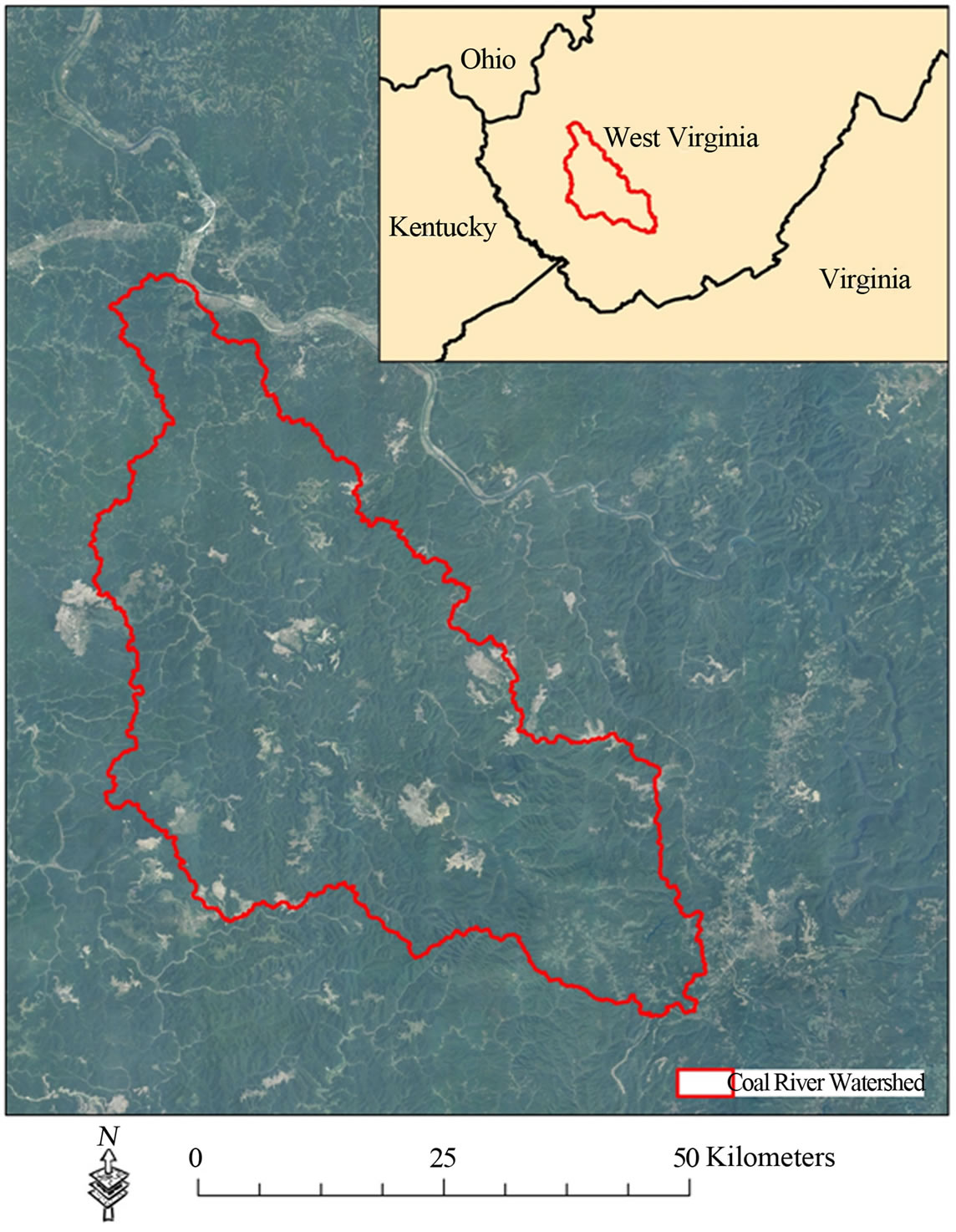
Figure 1. Study Area.
An interpolated raster surface was created from point data using ArcMap 10, and average point spacing of 0.01 m. Inverse distance weighting (IDW) was used to interpolate a raster surface since sample points were in an evenly distributed pattern. This process resulted in a 1 m resolution, floating point elevation dataset.
2.3. Assessing Landform Changes between 2003 and 2010
Landform changes were assessed in filled and cut or excavated areas resulting from mining and reclamation between 2003 and 2010. The 2010 LiDAR-derived DEM was compared to a 2003 photogrammetrically-derived DEM representing 2003 conditions. The 2003 DEM data were provided by the West Virginia Statewide Addressing and Mapping Board (SAMB) who contracted BAE Systems ADR to create a stereo photogrammetric-derived digital terrain model (DTM) from statewide, spring, leaf-off, 1:4800 scale aerial photography. The DEM was created in compliance with National Dataset standards (1/9th arc second) and produced from mass points and breaklines. This dataset supports a vertical accuracy of +/− 3.048 m, root mean square error (RMSE) and has a cell size of 3 m [20].
In order to match the resolution of the SAMB DEM, we resampled the LiDAR-derived raster to 3 m resolution using bilinear interpolation and snapped the grid to match the extent of the SAMB DEM. This process assured that the raster grids were completely aligned. This process resulted in two 3 m DEMs representing 2003 and 2010 conditions that could be compared. A vertical data transformation was unnecessary since both DEMs had a vertical reference of NAVD88 orthometric.
In order to detect systematic error between the 2003 and 2010 DEM data, a total of 281 points were collected in the field throughout the Coal River Watershed on flat, paved surfaces using Pacific Crest realtime kinematic (RTK) survey equipment. The elevation measurements from the 2003 and 2010 elevation raster data were obtained at these locations. The measurements from each DEM were then compared. The mean difference was −0.4 m with a maximum difference of 0.8 m and a minimum difference of −2.0 m. Based on this analysis we did not correct for systematic difference between DEMs.
Once DEMs were obtained, processed, and prepared, they were subtracted using Raster Calculator within the Spatial Analyst Extension of ArcMap [21]. This produced a grid of elevation differences throughout the watershed. Negative values indicated potential cuts or excavations while positive values indicated potential fills. However, difference could simply have resulted from errors in the DEMs or in methodology. As a result, once this elevation difference model was calculated, it was necessary to determine a tolerance or threshold that would constitute true change and not simply error or noise between the digital elevation datasets. The photogrammetric DEM had an error tolerance (RMSE) of +/− 3.048 m while the LiDAR DEM had and error tolerance of only 15 cm (0.15 m). An equation suggested by [22] was used to estimate this threshold. The RMSE of each dataset was squared, the results were summed, and the square root of the sum was then taken. The result was then multiplied by three to determine a cut off representing values that were greater than three standard deviations from the mean. This method assumes a Gaussian distribution. Elevation change measurements outside of this range were considered true elevation differences and not a result of error or noise. Reference [15] used the same methodology to derive an error tolerance for the analysis conducted in Perry County, Kentucky, USA.
According to this method, it is not certain whether differences less than +/− 9.2 m represented true topographic change. As a result, the elevation difference grid was reclassified so that values between −10 m and +10 m were considered no change, error between the DEMs, or noise. Pixels with values less than −10 m were considered potential cuts while pixels with values greater than 10 m were considered potential fills. This process produced a cut and fill mask.
A LULC dataset was created for the region from 2009 National Agriculture Imagery Program (NAIP) orthophotography. Optimally, imagery collected at the time of the LiDAR collection would have been utilized; however, such data were not available. The imagery was classified using an object-based feature extraction methodology, augmented with GIS decision rules and manual digitizing. Forest, grass, and barren land cover were extracted from the raw imagery.
Combining these data with mine permit boundaries from the West Virginia Department of Environmental Protection (WVDEP) made it possible to delineate barren and grassland land cover in mine permits. Grasslands in permits represent potential reclamation while barren areas represent areas of active mining or areas that have not yet been reclaimed. The extents of valley fill faces and slurry impoundments were digitized. According to an error assessment based on manual aerial photograph interpretation at 100 randomly selected points, the LULC dataset had an overall accuracy of 94% (KHat of 93%).
It was possible to further remove erroneous pixels as potential cut or fills by utilizing additional data, such as the high resolution land cover. For example, potential cut or fill pixels could be removed if they were outside of disturbance resulting from surface mining. The potential cut or fill pixels that existed within areas of mine disturbance (barren, grasslands, or valley fill faces) were considered. Slurry impoundments were excluded because of errors associated with water level. To complete this analysis, it was necessary to convert the raster data to polygons that represented contiguous areas of cut or fill. No smoothing or simplification was applied.
Small areas of topographic change could also be removed as error or noise. Thresholds were determined from the hand digitized valley fill faces. The average size of these faces was 73,257 m2 (7.3 ha) with a standard deviation of 67,013 m2 (6.7 ha). Based from this distribution, any contiguous area of cut or fill that was smaller than 60,000 m2 (6 ha) was considered noise and removed. Although this threshold was somewhat arbitrary, it was selected since this study focused on detecting large expanses of excavation and fills.
The result of this analysis was a vector layer of potential cut or fill extents in which topographic change had occurred between 2003 and 2010. The extents were used to define areas of potential terrain change for analysis and comparison of the distributions of landforms. Although there was error associated with this methodology, it was adequate for this analysis since we were not interested in conducting an assessment of absolute elevation change or volumetric change but in defining areas in which to compare categorical terrain data and their impact on forest communities.
2.4. Creation of Landforms
The DEM data were used to classify the terrain into the following landforms: cliff, steep slope, slope crest, upper slope, flat summit, sideslope, cove, dry flat, moist flat, wet flat, and slope bottom. The methodology described by [17] provides a means to utilize DEM data to classify the landscape into different units of ecological significance. DEM derivatives including slope in degrees, a hydrologically filled DEM, flow direction, and flow accumulation were created using ArcMap 10. The slope and flow accumulation grids were utilized to calculate a moisture index. The moisture index is a relative measure of the moisture of a specific cell, and it assumes that the moisture level is a function of how much water flows into the cell, predicted by flow accumulation, and how fast the water can flow out, described by slope [20-25].
Landscape position was calculated following [26] to divide the landscape into the following categories: ridge, wide ridge, slope/flat, slope/cove. The approach is based on a local neighborhood analysis of elevation values in which a cell is compared to the mean elevation of all values within 3 by 3 windows. Landscape position was combined with slope and moisture index data to derive the final landform classes. This procedure was conducted for both the 2003 and the 2010 DEMs. The comparisons of the derived landforms included:
• Areas filled between 2003 and 2010 (mining related);
• Areas cut or excavated between 2003 and 2010 (mining related);
• Areas of mine reclamation in 2009, areas of mining disturbance or reclamation in 2009, and areas in WVDEP mine permits but not disturbed (forested in 2009).
This enabled the comparison of post-mining landform categories with pre-mining conditions.
3. RESULTS
Figure 2 shows the distribution of landforms in a MTR/VF site representing 2010 conditions. Comparing the mine site with the surrounding landscape, the distribution of landforms is greatly altered by mining even after reclamation has occurred. Figure 3 shows a different MTR/VF site and offers a comparison of landforms within areas cut or filled between 2003 and 2010, and
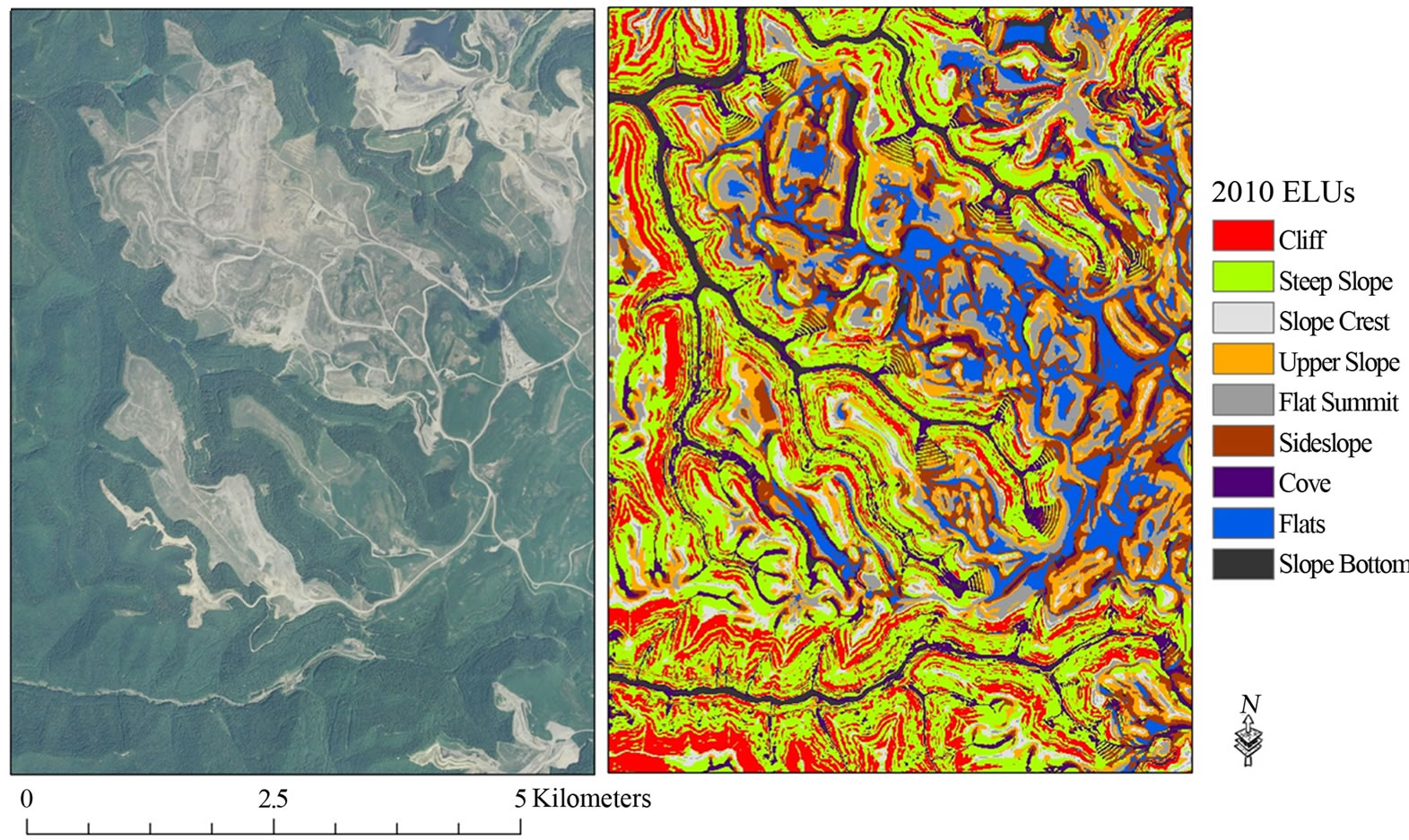
Figure 2. Example of landform distribution after landscape alteration and MTR/VF. The imagery is orthophotography representing growing season 2011 conditions.
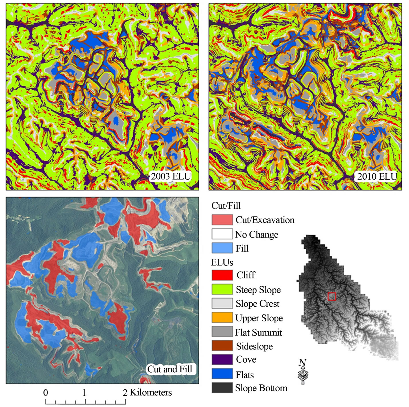
Figure 3. Comparison of landforms at mine site. The imagery is orthophotography representing growing season 2011 conditions.
this visualization also shows a redistribution of landforms.
Landforms were compared for areas of cut or fill between 2003 and 2009 within mine disturbance. Such areas represent potential areas of true topographic change. The results are described in Tables 1 and 2 and Figures 4 and 5. Chi-square tests were performed on the categorical data for this observational study, and the results suggest a statistically different distribution of landforms after volumetric change (α = 0.001).
It was possible that differences in the DEM production methodology could have resulted in differences in the resulting landform classification. This was observed by visual inspection of the results and was a source of error in the data represented in Figures 4 and 5. As a result, differences in classification and distribution of landforms could result from true terrain change or could be a product of the differences in DEM production methodology, photogrammetric or LiDAR-derived. In order to resolve such ambiguity, terrain classification differences were assessed for different surface mining LULC categories (2009) using the 2010 ELU data only. The results are described in Table 3 and Figure 6 in which landform classes were compared for areas in mine permits but still forested or not disturbed, areas of mine reclamation, and areas of mine reclamation or mining disturbance. The assumption was that areas permitted for surface mining should generally have similar topography. As a result, undisturbed areas within the mine permits representing pre-mining terrain were compared to mined or reclaimed areas representing post-mining terrain. This analysis showed a marked change in landforms from steep slopes to more flat topography, such as moist flats, upper slopes, and flat summits. We argue this, this is a more valid method to assess topographic change induced by surface mining and excavation because this technique was not impacted by differences in DEM methodology.
A chi-square test was performed to test for a statistical difference in the distributions of landforms associated with Table 3 and Figure 6. The test suggest a statistically significantly different categorical distribution of landforms preand post-mining (α = 0.001). The landform classes were then reclassified to only slopes and flats, and a second chi-square test suggests a statistically significant increase in flats and decrease in slopes postmining (α = 0.001).
Two sample Student’s t-tests were used to determine if preand post-mining average slope conditions were statistically different. A comparison of slopes for all pixels in areas that were not mined in 2003 but were predicted as reclaimed relative to summer 2009 conditions showed a statistically significant different average slope at the 99.9% confidence level. However, as noted above, difference could have been a result of different methodol-
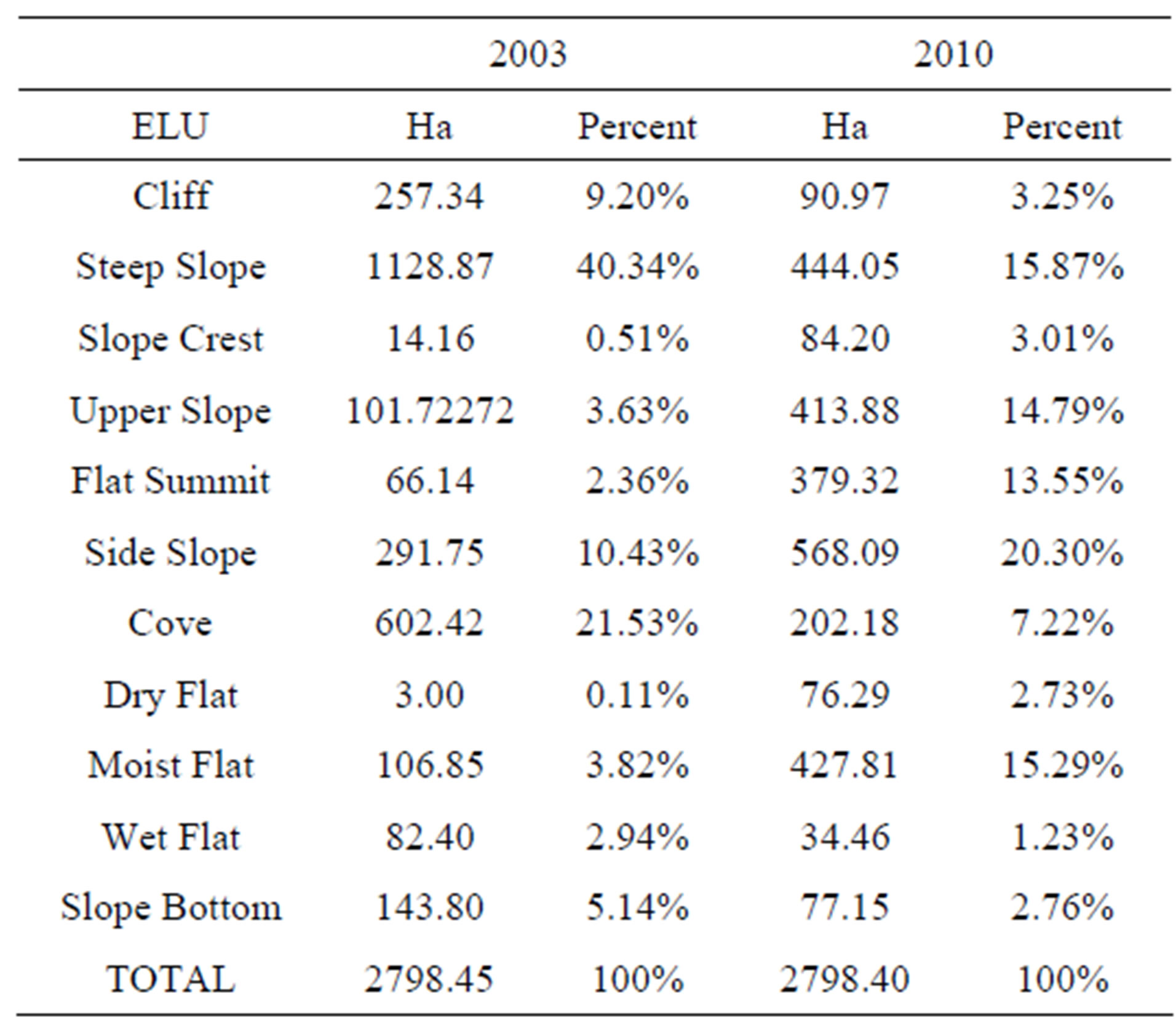
Table 1. Distribution of landforms for areas within mines and filled between 2003 and 2010.
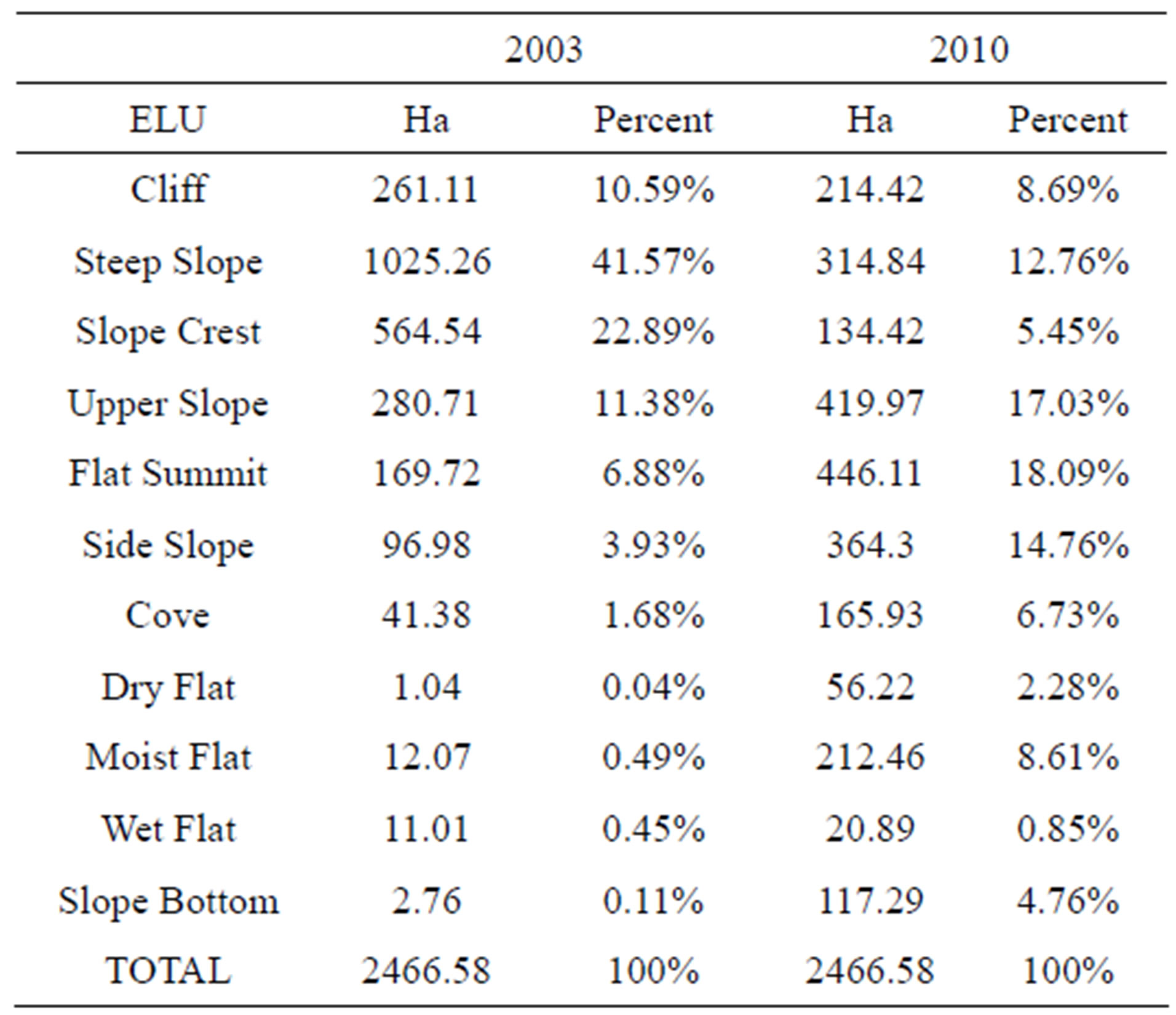
Table 2. Distribution of landforms for areas within mines and cut or excavated between 2003 and 2010.
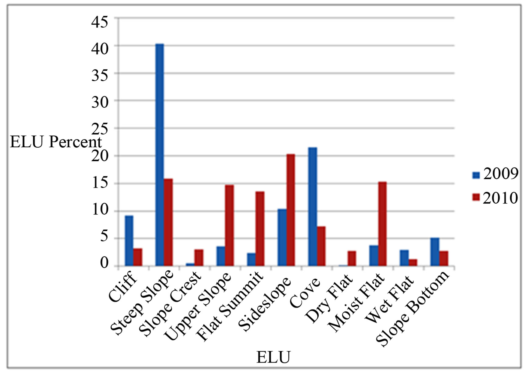
Figure 4. Comparison of landforms for areas within mines and filled between 2003 and 2010.
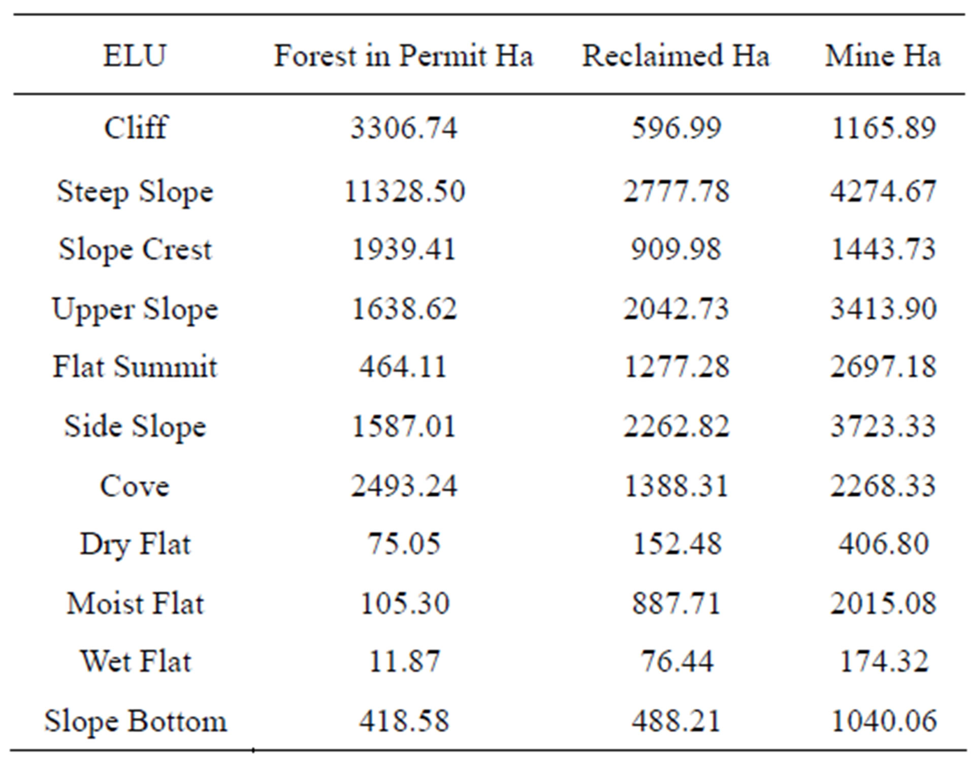
Table 3. Distribution of landforms within different land cover categories (2009) relative to 2010 DEM.
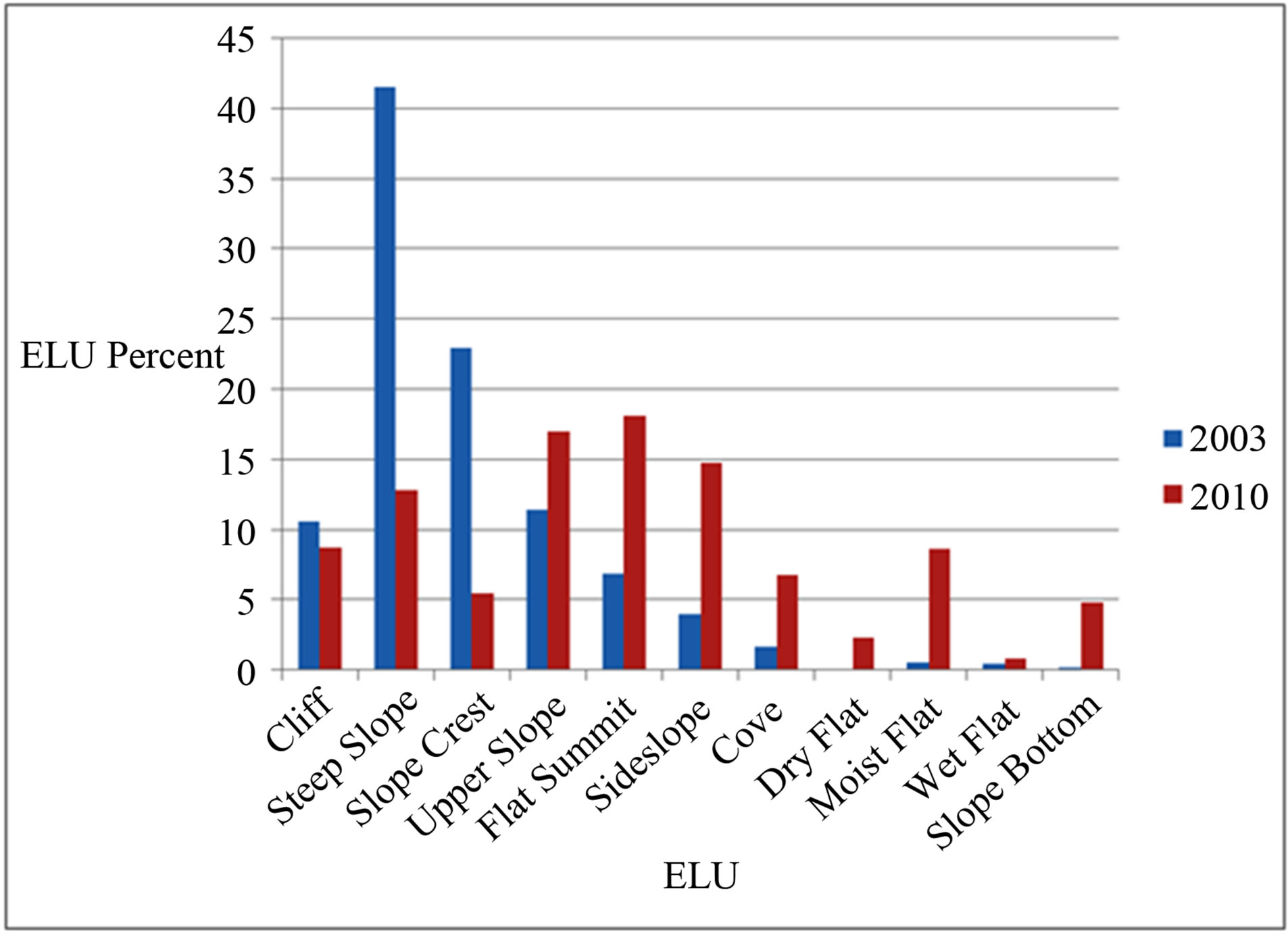
Figure 5. Comparison between landforms for areas within mines and cut or excavated between 2003 and 2010.
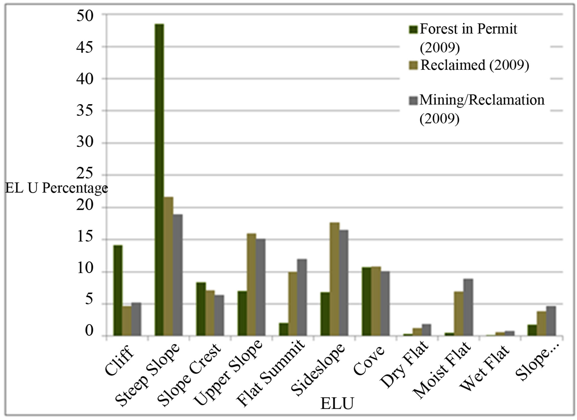
Figure 6. Comparison of landforms within different land cover categories 2009 relative to 2010 DEM.
ogy utilized to produce the DEM data. As a result, we also compared all pixels that were forested in permits, relative to growing season 2009 conditions, and areas that were either reclaimed or mined disturbed or reclaimed.
4. DISCUSSION
The Southern Coalfields of West Virginia are characterized by steep slopes and narrow valleys [19]; however, this description often does not accurately describe the post-mining terrain and geomorphology. This study helped to indicate the specific landform classes that are altered in our representative study area.
The geomorphic complexity and steep slopes that characterize this region contribute to the biological richness of the Appalachian Plateau and the mixed mesophytic forest biogeographic region [27]. The Southern Coalfields of West Virginia exists within one of the most biodiverse regions within the temperate zone, and more than 2000 vascular plants exist on the landscape [28,29]. This region is globally recognized as significant for biodiversity conservation [30]. The variety of forest types is in part a result of the elevation changes and steep topography of this landscape [27].
There has been a shift in focus from rare or endangered species management to ecosystem and landscapescale management, which requires that a diversity of ecological processes be considered [31]. The methodology of this study provides an opportunity to understand landscape and terrain alterations and the ability now to examine the critical links of landforms to terrestrial habitat, ecosystem health, and biodiversity.
The question arises as to how this terrain alteration will impact biodiversity and ecosystem health. If forests are reestablished on these topographically altered mountaintops, will pre-mining forest communities and ecosystems be reestablished? Although traditional reclamation often results in grasslands or scrub/shrub lands on the reclaimed and topographically altered mountaintops [6,32] has suggested a forest reclamation approach that includes the creation of soils to support a forest community, loose grading to avoid soil compaction and increased bulk density, use of less competitive ground cover to allow for forest growth, planting of a wider variety of trees and native species, and use of proper tree planting techniques to aid in reforestation of mine scarred lands. This technique is being more commonly implemented to reclaim mine disturbed areas [32]. If such methodology is successful at creating stable and mature forest communities, will these forests represent pre-mining conditions or serve the same ecological function if the topography has been greatly altered? This question is yet to be fully explored. Assuming that topographic factors, such as slope and landscape position, are correlated with forest community type as described by [33], we suggest that it is reasonable to assume that topographic changes will result in forest community changes, and forest community variety and distribution are related to biodiversity as suggested by [27]. Terrain alteration should be considered along with the impact of introducing non-forest edge and disrupting the interior nature of the forest since MTR/VF has been shown to have the potential to alter community faunal composition [34].
5. SUMMARY
This study identified specific landform classes that were impacted due to cut/excavation or filled material at surface mined sites in a West Virginia, USA watershed. The landform analysis methodology provided a means to quantify and spatially assess terrain alterations using categorical landscape data derived from DEMs, a potential first step for assessing the impact of MTR/VF on terrestrial habitat and ecosystems at the landscape scale. Research is needed to understand the relationship between terrain and forest communities in the Appalachian region at both the local and regional scales. A more complete understanding of these relationships may aid in an understanding of the impact of MTR/VF on forest communities, terrestrial habitat, ecosystem health, and biodiversity.
6. ACKNOWLEDGEMENTS
This study was sponsored by the Appalachian Research Initiative for Environmental Science (ARIES). ARIES is an industrial affiliates program at Virginia Tech, Blacksburg, VA, USA, supported by members that include companies in the energy sector. The research under ARIES is conducted by independent researchers in accordance with the policies on scientific integrity of their institutions. The views, opinions and recommendations expressed herein are solely those of the authors and do not imply any endorsement by ARIES employees, other ARIES-affiliated researchers or industrial members. Information about ARIES can be found at http://www.energy.vt.edu/ARIES.
We would also like to acknowledge funding support provided by US Environmental Protection Agency and the West Virginia Experiment Station. This work was completed with the assistance of Adam Riley, Elise Austin, and Charles Yuill who are Remote Sensing Analyst, GIS Analyst and Landscape Analyst respectively at West Virginia University.
Lastly, we thank the anonymous reviewers who helped to improve the manuscript.
REFERENCES
- Hooke, R.L. (1994) On the efficacy of humans as geomorphic agents. GSA Today, 4, 224-225.
- Saylor, K.L. (2008) Land cover trends project: Central Appalachians. US Department of the Interior, Washington. http://landcovertrends.usgs.gov/east/eco69Report.html
- Drummond, M.A. and Loveland T.R. (2010) Land-use pressure and a transition to forest-cover loss in the eastern United States. BioScience, 60, 286-298. doi:10.1525/bio.2010.60.4.7
- Townsend, P.A., Helmers, D.P., Kingdon, C.C., McNeil, B.E., de Beurs, K.M. and Eshleman, K.N. (2009) Changes in the extent of surface mining and reclamation in the Central Appalachians detected using a 1976-2006. Landsat time series. Remote Sensing of Environment, 113, 62- 72. doi:10.1016/j.rse.2008.08.012
- Palmer, M.A., Bernhardt, E.S., Schlesinger, W.H., Eshleman, K.N., Fourfoula-Georgiou, E., Hendryx, M.S., Lemly, A.D., Likens, G.E., Loucks, O.L., Power, M.E., White, P.S. and Wilcock, P.R. (2010) Mountaintop mining consequences. Science, 327, 148-149. doi:10.1126/science.1180543
- Simmons, J.A., Currie, W.S., Eshleman, K.N., Kuers, K., Monteleone, S., Negley, T.L., Pohlad, B.R. and Thomas, C.L. (2008) Forest to reclaimed mine land use change leads to altered ecosystem structure and function. Ecological Applications, 18, 104-118. doi:10.1890/07-1117.1
- Wickham, J.D., Ritters, K.H., Wade, T.G., Coan M. and Homer, C. (2007) The effect of Appalachian mountaintop mining on interior forest. Landscape Ecology, 22, 179- 187. doi:10.1007/s10980-006-9040-z
- Bernhardt, E.S. and Palmer, M.A. (2011) The environmental costs of mountaintop mining valley fill operations for aquatic ecosystems of the Central Appalachians. Annals of the New York Academy of Sciences, 1223, 39-57.
- USEPA (2005) Mountaintop mining/valley fills in Appalachia. Final programmatic environmental impact statement. Region 3, US Environmental Protection Agency, Philadelphia. http://www.epa.gov/region3/mtntop/index.htm
- Fox, J.F. and Campbell, J.E. (2009) Terrestrial carbon disturbance from mountaintop mining increases lifecycle emissions for clean coal. Environmental Science and Technology, 44, 2144-2149. doi:10.1021/es903301j
- Hooke, R.L. (1999) Spatial distribution of human geomorphic activity in the Unites States: Comparison with rivers. Earth Surface Processes and Landforms, 24, 687- 692. doi:10.1002/(SICI)1096-9837(199908)24:8<687::AID-ESP991>3.0.CO;2-#
- Fritz, K.M., Fulton, S., Johnson, B.R., Barton, C.D., Jack, J.D., Word, D.A. and Burke, R.A. (2010) Structural and functional characterisitcs of natural and constructed channels draining a reclaimed mountaintop removal and valley fill coal mine. Journal of the North American Benthological Society, 29, 673-689. doi:10.1899/09-060.1
- Larson, C.F., Motyka, R.J., Arendt, A.A., Echelmeyer, K.A. and Geissler, P.E. (2007) Glacier changes in southeast Alaska and northwest British Columbia and contribution to sea level rise. Journal of Geophysical Research, 112, F01007.
- Woolard, J.W. and Colby, J.D. (2002) Spatial characterization, resolution, and volumetric change of coastal dunes using airborne LiDAR: Cape Hatteras, North Carolina. Geomorphology, 48, 269-287. doi:10.1016/S0169-555X(02)00185-X
- Gesch, D.B. (2005) Analysis of multi-temporal geospatial data sets to assess the landscape effects of surface mining. National Meeting of the American Society of Mining and Reclamation, ASMR, Lexington, 415-432.
- Shank, M. (2004) Development of a mining fill inventtory from multi-date elevation data. Advanced Integration of Geospatial Technologies in Mining and Reclamation, Surface Mining Reclamation and Enforcement, Technical Innovation and Professional Services, Denver, 1-16. http://gis.dep.wv.gov/tagis/projects/valley_fill_paper.pdf
- Anderson, M.G., Merrill, M.D. and Biasi, F.B. (1998) Connecticut River Watershed analysis: Ecological communities and neo-tropical migratory birds. Eastern Conservation Science. The Nature Conservancy, 36.
- WVGES (West Virginia Geologic and Economic Survey) (2005) Physiographic provinces of West Virginia. http://www.wvgs.wvnet.edu/www/maps/pprovinces.htm
- Strausbaugh, P.D. and Core, E.L. (1977) Flora of West Virginia. Seneca Books Inc. Morgantown, 1079.
- Grayson, R.B., Moore, I.D. and McMahon, T.A. (1992) Physically based hydrologic modeling: 1. A terrain-based model for investigative purposes. Water Resources Research, 28, 2639-2658. doi:10.1029/92WR01258
- Environmental Systems Research Institute (ESRI) (2010) ArcGIS ArcMap Version 10.0. Redlands.
- Moore, D.M., Lees, B.G. and Davey, S.M. (1991) A new method for predicting vegetation distributions using decision tree analysis in a geographic information system. Environmental Management, 15, 59-71. doi:10.1007/BF02393838
- Boer, M., Del Barrio, G. and Puigdefabregas, J. (1996) Mapping soil depth classes in dry Mediterranean areas using terrain attributes derived from digital elevation models. Geoderma, 72, 99-118. doi:10.1016/0016-7061(96)00024-9
- O’Loughlin, E.M. (1986) Prediction of surface saturation zones in natural catchments by topographic analysis. Water Resources Research, 22, 794-804. doi:10.1029/WR022i005p00794
- Parker, A.J. (1982) The topographic relative moisture index: An approach to soil-moisture assessment in mountain terrain, Physical Geography, 3, 160-168.
- Fels, J. and Zobel, R. (1995) Landscape position and classified landtype mapping for the statewide DRASTIC mapping project. North Carolina State University, Raleigh, 1-8.
- Hinkle, C.R., McComb, W.C., Safely, J.M. Jr. and Schmalzer, P.A. (1993) Mixed mesophytic forests. In: Martin, W.H., Boyce, S.C. and Echternacth, A.C., Eds., Wiley, New York, 203-253.
- Master, L.L., Flack, S.R. and Stein, B.A. (1998) Rivers of life: Critical watersheds for protecting freshwater biodiversity. Then Nature Conservancy, Arlington.
- Stein, B.A., Kutner, L.S., and Adams, J.S. (2000) Precious heritage: The status of biodiversity in the united states. Oxford University Press, New York.
- Ricketts, T.H., Dinerstein, E., Olson, D.M., Loucks C.J., Eichbaum, W., DellaSala, D., Kavanagh, K., Hedao, P., Hurley, P.T., Carney, K.M., Abell, R. and Walters, S. (1999) Terrestrial ecoregions of North America: A conservation perspective. Island Press, Washington.
- Poiani, K.A., Richter, B.D., Anderson, M.G. and Richter, H.E. (2000) Biodiversity conservation at multiple scales: Functional sites, landscapes, and networks. American Institute of Biological Sciences, 50, 133-146.
- Zipper, C.A., Burger, J.A., Skousen, J.G., Angle, P.N., Barton, C.D., Davis, V. and Franklin, J.A. (2011) Resorting forests and associated goods and services on Appalachian coal surface mines. Environmental Management, 47, 751-765. doi:10.1007/s00267-011-9670-z
- Whittaker, R.H. (1956) Vegetation of the great smoky mountains. Ecological Monographs, 26, 1-80. doi:10.2307/1943577
- USEPA (US Environmental Protection Agency) (2003) Draft programmatic environmental impact statement on mountaintop mining/valley fills in Appalachia. http://www.epa.gov/region3/mtntop/eis2003.htm