Natural Science
Vol.4 No.2(2012), Article ID:17322,6 pages DOI:10.4236/ns.2012.42013
Deformation prediction model of surrounding rock based on GA-LSSVM-markov
![]()
Engineering Institute of Corps of Engineers, PLA University of Science & Technology, Nanjing, China; *Corresponding Author: diandian2829@163.com
Received 2 January 2012; revised 8 February 2012; accepted 12 February 2012
Keywords: Genetic Algorithm (GA); Least Square Support Vector Machines (LSSVM); Markov; Evaluation; Surrounding Rock; Command Protection Engineering
ABSTRACT
Command protection engineering is the important component of national protection engineering system. To raise the level of its construction, a deformation prediction model is given based on Genetic Algorithm (GA), Least Square Support Vector Machines (LSSVM) and markov theory. Genetic algorithm is used to improve the parameter of LSSVM. Markov predict method is used to improve the precision of the prediction model. Finally, be used to a certain command protection engineering, the accuracy of the algorithm is improved obviously. The model is proved to be credible and precise.
1. INTRODUCTION
Surrounding rock deformation is a complex nonlinear process [1]. Surrounding rock deformation monitoring, as basic information of evaluation and reflect of the surrounding rock change, its production, development and change can be regarded as time series. Model with the monitoring displacement values, can be used to predict its development trend in the future, to grasp the changing law of rock, which is very important in engineering [2,3].
In the field of surrounding rock deformation prediction, in order to objectively reflect the rules between time and change, mathematics method or mathematical model is often need, used to prediction analysis. At present, a lot of research is given, common method are as follows, Lagrange interpolation method, exponential smoothing, the spline interpolation method, regression model method, time series analysis, gray system theory, the artificial neural network method, the response surface treatment technology and chaos phase space reconstruction processing technology, etc. [4]. Research method on time series contains, polynomial regression, gray theory, the neural network and genetic neural network method etc [5-10]. The methods have made certain effects. But these methods usually have good effect only when the dependent and independent variable is linear relationship or some simple function relationship. When datum are little and have no statistical significance, the above methods can’t be used.
Support vector machine, with the foundation of structural risk minimization principle, has advantages that the others, with the foundation of empirical risk minimizetion principle, have not [11]. The relationship of the dependent and independent variable can’t be learned. The complex mapping relationship can be learned from the sample. At the same time, model can be built with fewer samples. Some research is given on the surrounding rock deformation prediction with support vector machine (SVM) [12,13]. The accuracy of the models is not very good. In this paper, Least Square Support Vector machine (LSSVM) is improved with the method of Genetic Algorithm (GA), markov forecast method. The method is used to give research on surrounding rock deformation prediction of command protection engineering.
2. DEFORMATION PREDICTION MODEL BASED ON GA-LSSVM-MARKOV
2.1. LSSVM Prediction Model
For nonlinear rock deformation sequence of command protection engineering, a time series  can be got through the monitoring. To predict the nonlinear deformation sequence, is to find the relationship of
 , as deformation value of time
 , and
, and , as the deformation value of the p times before, that is
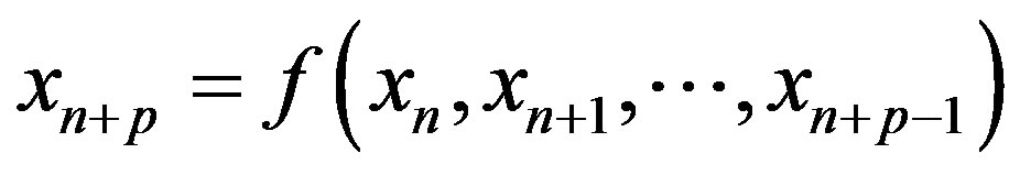 .
.  is a nonlinear function, indicates nonlinear relationship between deformation sequences.
Based on support vector machine theory, the nonlinear relationship above can be got with the support vector machine to learn  deformation sequences
 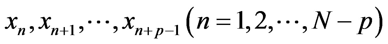 . In LSSVM, x is mapped to high dimension space through
 . Then linear regression function is constructed in the feature space as follows.
 (1)
(1)
In the formula,  is weight vectors,
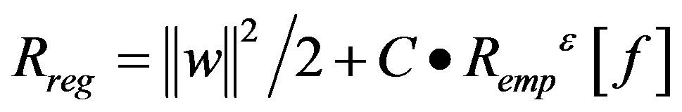
  is bias. Solve of the formula boils down to minimize the risk structure as follows:
 (2)
(2)
In the formula,  is depicting incredible range,
  is experienced risk, C > 0 is factor of balance experience risk and the confidence range. If
  uses no sensitive loss function, and considers allowing error, LSSVM model can be got as follows.
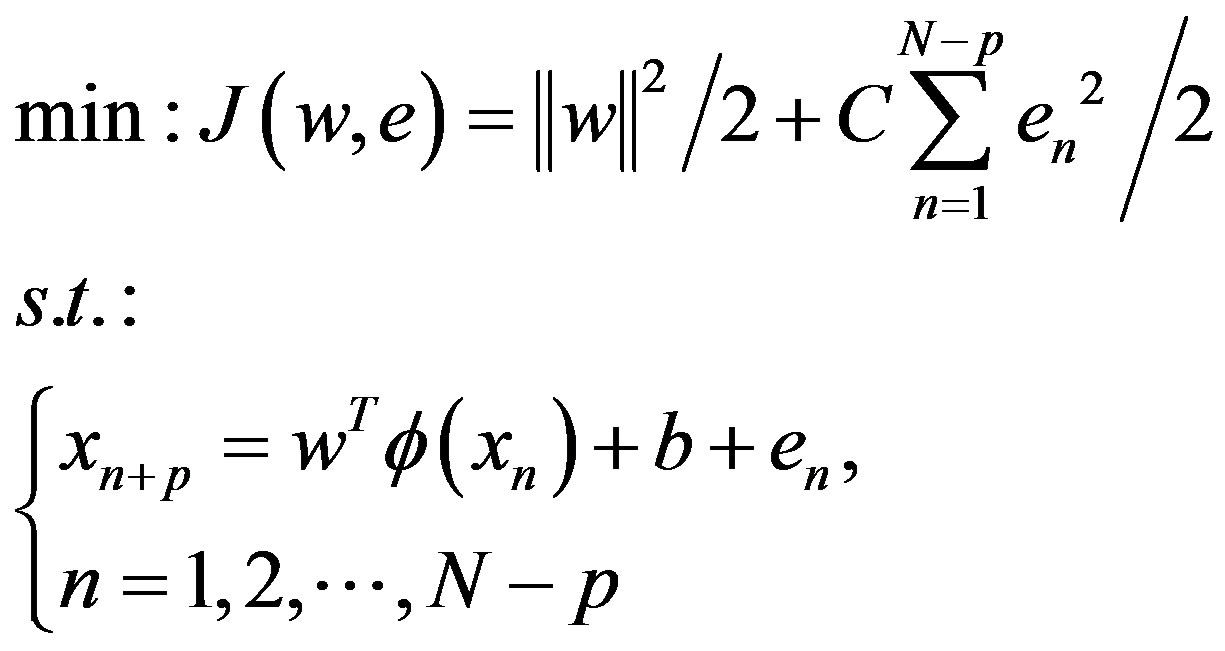 (3)
(3)
To solve the optimization problem, the constrained problem is changed to unconstrained problem. Lagrange function is built as follows:
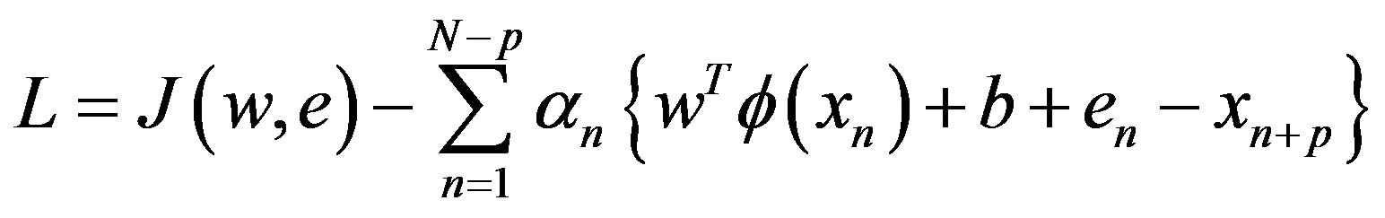 (4)
(4)
Then, due to the KKT condition, there are formulae as follows:
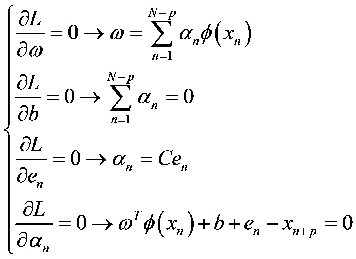 (5)
(5)
Eliminate  and
and , there is formula as follows:
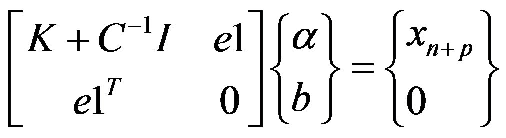 (6)
(6)
 , I is
  order unit array,
  , K is kernel function matrix, its element is as follows:
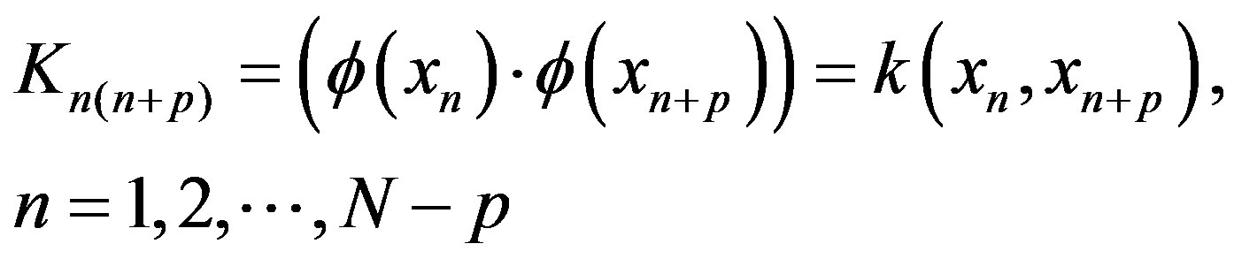 (7)
(7)
To solve the linear equations, the output of LSSVM is as follows:
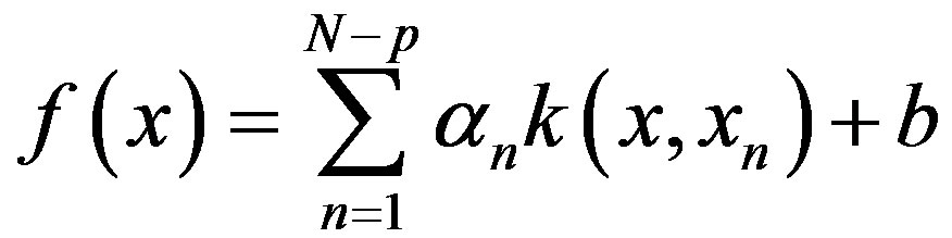 (8)
(8)
Compared to the standard SVM model, the solution of LSSVM is easier and faster.
2.2. Parameter Optimization of LSSVM with GA
The Genetic algorithm is a highly parallel, random and adaptive optimization algorithm. The solution space of optimization problem is mapped to genetic coding arrays, and each possible solution is expressed as a chromosome, which is consisting of genes. Each chromosome represents a solution; a number of chromosomes are a group. Firstly, initial population is random generated. The fitness of each chromosome environment is calculated due to the fitness function determined by the objective function, and then the next generation of groups is copied according to the fitness of chromosomes, and crossover, mutation etc. Repeatedly from generation to generation, the most convergence group which is adapting to the environment is got finally. And the optimum solution of the problem is obtained [14].
The process that genetic algorithm is used to optimize parameters of the least square support vector machine are as follows:
Step 1: set the initial value, such as the initial population scale N, the maximum genetic algebra T, the crossover probability Pc and the mutation probability Pm, etc.
Step 2: give binary code to the parameters to be optimized, random generate the initial population.
Step 3: calculate the fitness of individuals in the population.
Step 4: according to individual fitness, select individual to the next generation according with certain probability Ps (choose probability) to certain rules (the roulette method in this paper).
Step 5: select two individual of group as parent body, have two new individual on cross operation with certain probability Pc (crossover probability).
Step 6: random select individuals in the group on variation operation with certain probability Pm (mutation probability). Through random change some of the individual genes, produce the new individual.
Step 7: termination conditions judgment. If t ≤ T, turned to Step 2; If t > T or average fitness value is less than a constant changes over a certain algebra, the algorithm is terminated.
Step 8: to decode the optimal solution, the optimized parameters can be got.
2.3. Markov Optimization Method
Markov theory is the core of the stochastic process theory. Markov process is a category of random process which is suitable for a wide range of area. Because its model is concise and can seize the nature of things, it is a particularly important special stochastic process. Markov predict is an analysis method which applies the state transfer rule of system, and analyzes changing trends and future development of random events, and provides the decision makers information. It reveals the future development trend of system based on the system state transition probability [15-17].
2.3.1. The State Division
Regard the different fluctuation threshold between the displacement measurement values and LSSVM fitting relative error as state division standard. Divide the time series into several state, notes for S1, S2, ∙∙∙ , Sm, ∙∙∙ , SM, M stands for state number. The upper and lower value of threshold forms are as formula 9, and the average relative error  are as formula 10.
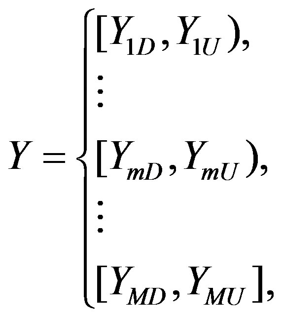 (9)
(9)
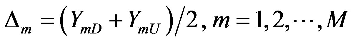 (10)
(10)
2.3.2. The State Transition Probability Matrix Calculation
Set the number of state Si in the sequence as , and the number that state Si transfers to Sj by k steps as
 , the displacement probability as follows:
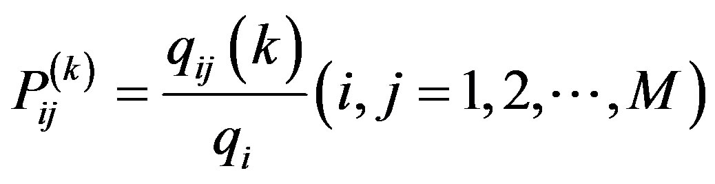 (11)
(11)
Because the last state displace uncertainly, the last k ones should be removed from .
.
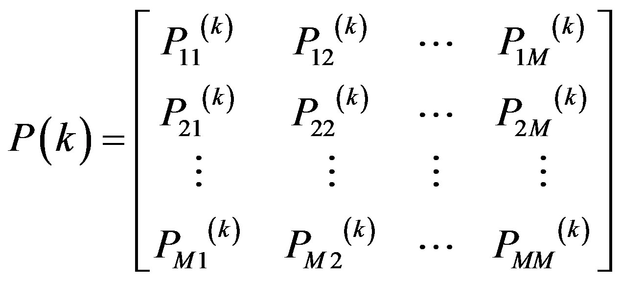
Through calculating the state transition probability, the state displacement transition matrix can be built as follows.
2.3.3. The Predict Table
Based on the state transition matrix , the future direction of the system can be predicted. Firstly, the predict table should be built. The method is as follows. Choose the recent n measured step from predict one, according to the distance away from the predict step, we set transfer steps as 1, 2, ∙∙∙ , M. In the transfer matrix of the corresponding number, the new probability matrix can be constituted with the row vector of start states. If the column vector of new probability matrix is summated, the probability of next step possible error state Sm can be got as pm.
If the future displacement of time series is confirmed, the change interval of prediction can be confirmed. Take displacement error  of time series as the weighted average of the values of the state errors. Then the most likely prediction of the sequence is as follows:
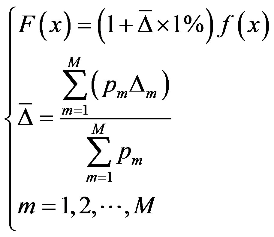 (12)
(12)
F(x) stands for the improved prediction by markov, and f(x) stands for LSSVM prediction.
If we join up formulae 10 and 12, the improved predictive value by markov can be got.
2.3.4. Dynamic Rolling Prediction
When the measure of step n is obtained, we delete the first step of data and supple n + 1 step of data, and form new learning samples. It ensures that the latest observation data can be used in predict every time. Continue to step 1 - 3.
2.4. GA-LSSVM-Markov Prediction Model
The flow sheet of GA-LSSVM-markov prediction model is in Figure 1.
3. EXAMPLE
There is an example about certain command protection engineering. The monitoring displacement data are in Table 1. The interval is about a month, and there are 30 steps.
3.1. GA-LSSVM Displacement Fitting
Related parameters of GA algorithm are: stop condition are ε < 0.001 or maximum evolution is 1000, population size of algebra is 30. Parameters of support vector machine are: the value range of C is [0,100], the value range of g is [0,100]. After trying calculating, we choose C = 86.5122, g = 28.169, s = 3, p = 0.01. 26 learning samples are constructed by first 26 time step, and the last four time step is inspection samples.
In Table 2, the measured displacement values, LSSVM fitted values, and absolute errors and relative error of 26 initial samples are listed. In Table 3, the measured displacement values, LSSVM predicted values, absolute
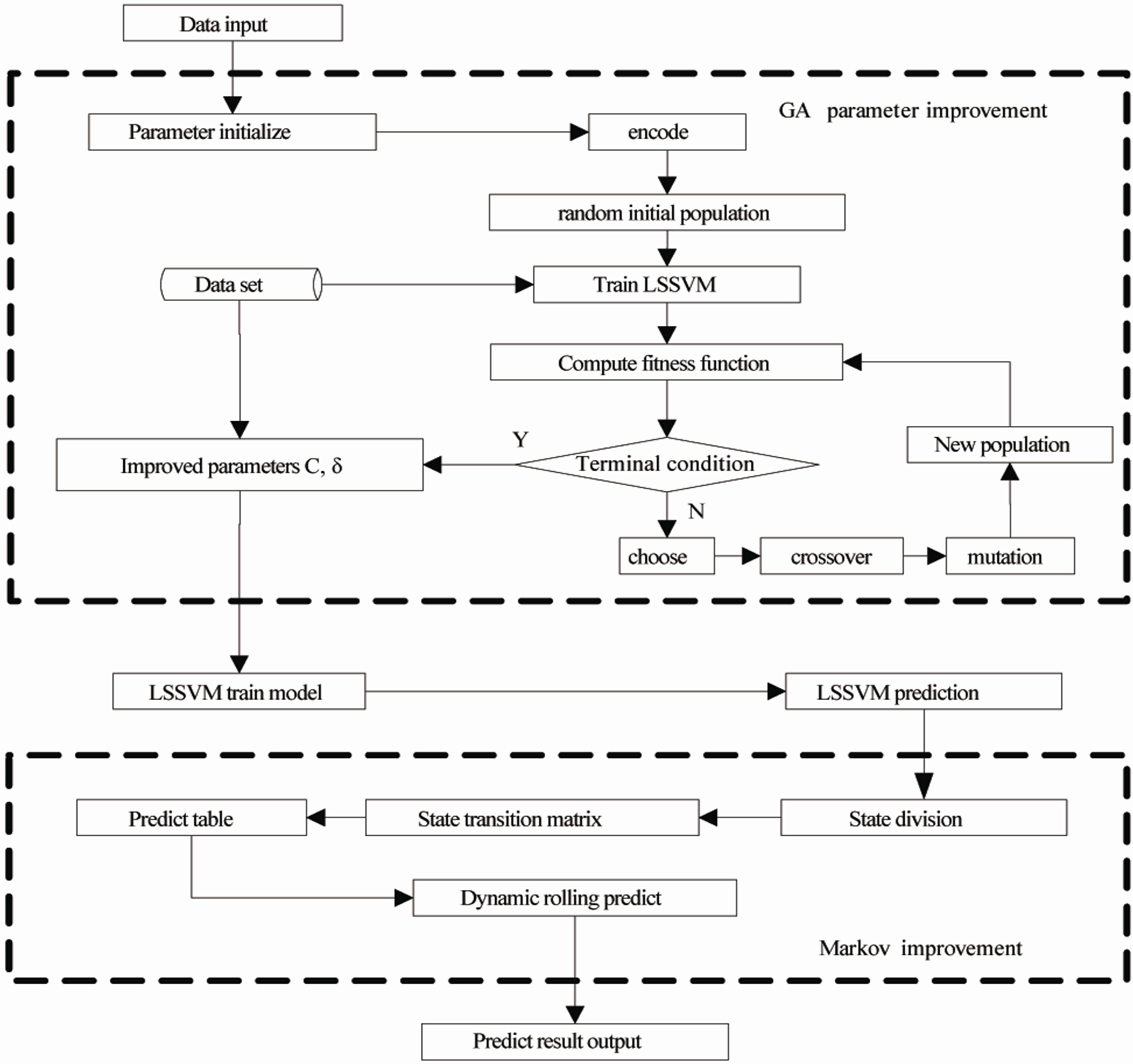
Figure 1. The flow sheet of GA-LSSVM-markov prediction model.
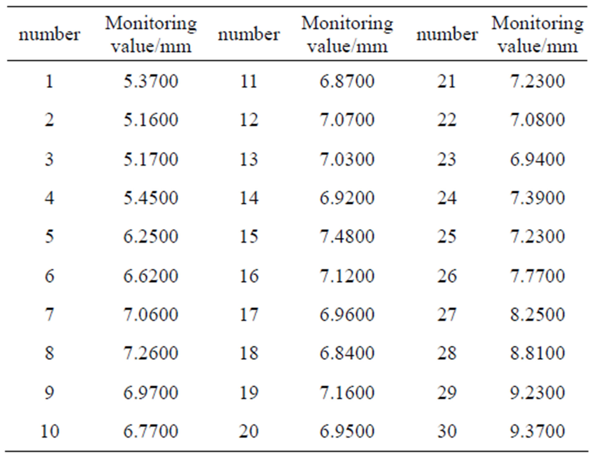
Table 1. Monitoring displacement datum of certain command protection engineering.
errors and relative error of 4 test samples are listed. The average of relative error absolute value is 1.2614. The accuracy of prediction is distinctly improved, compared to the results in reference [3.11] [3.12].
In Figure 2, the measured displacement values and LSSVM predicted values of learning samples and test samples are compared separately.
3.2. Markov Improvement of Prediction
3.2.1. The State Division
The state division standard is in Table 4. According to the standard, the state division results are in Table 2, Table 3.
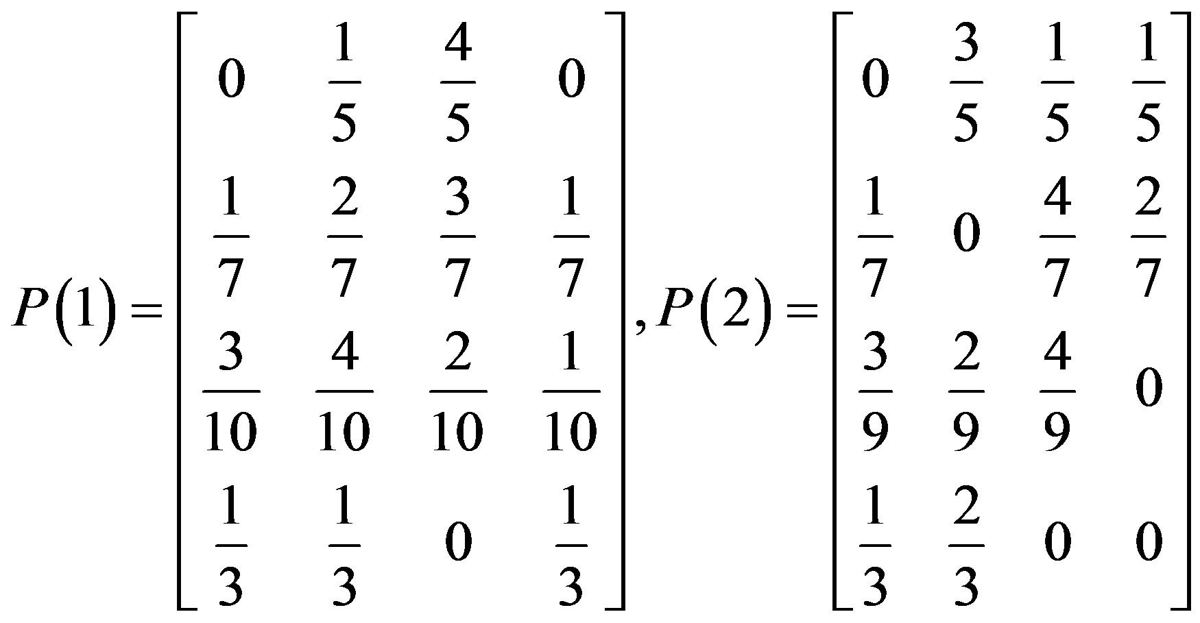
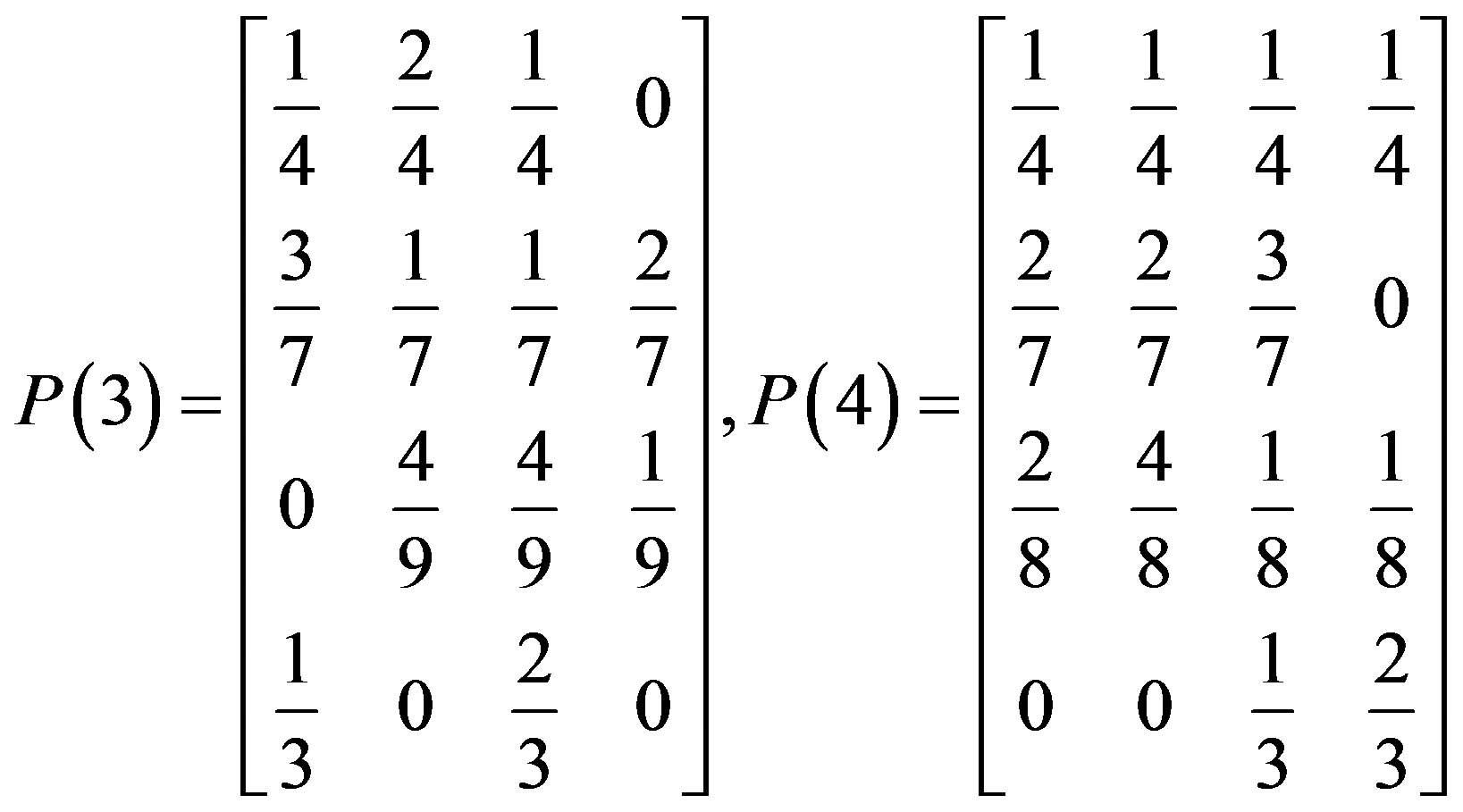
3.2.2. The State Transition Probability Matrix
According to the states in Table 1 and formula 12, the state transition probability matrixes are as follows:
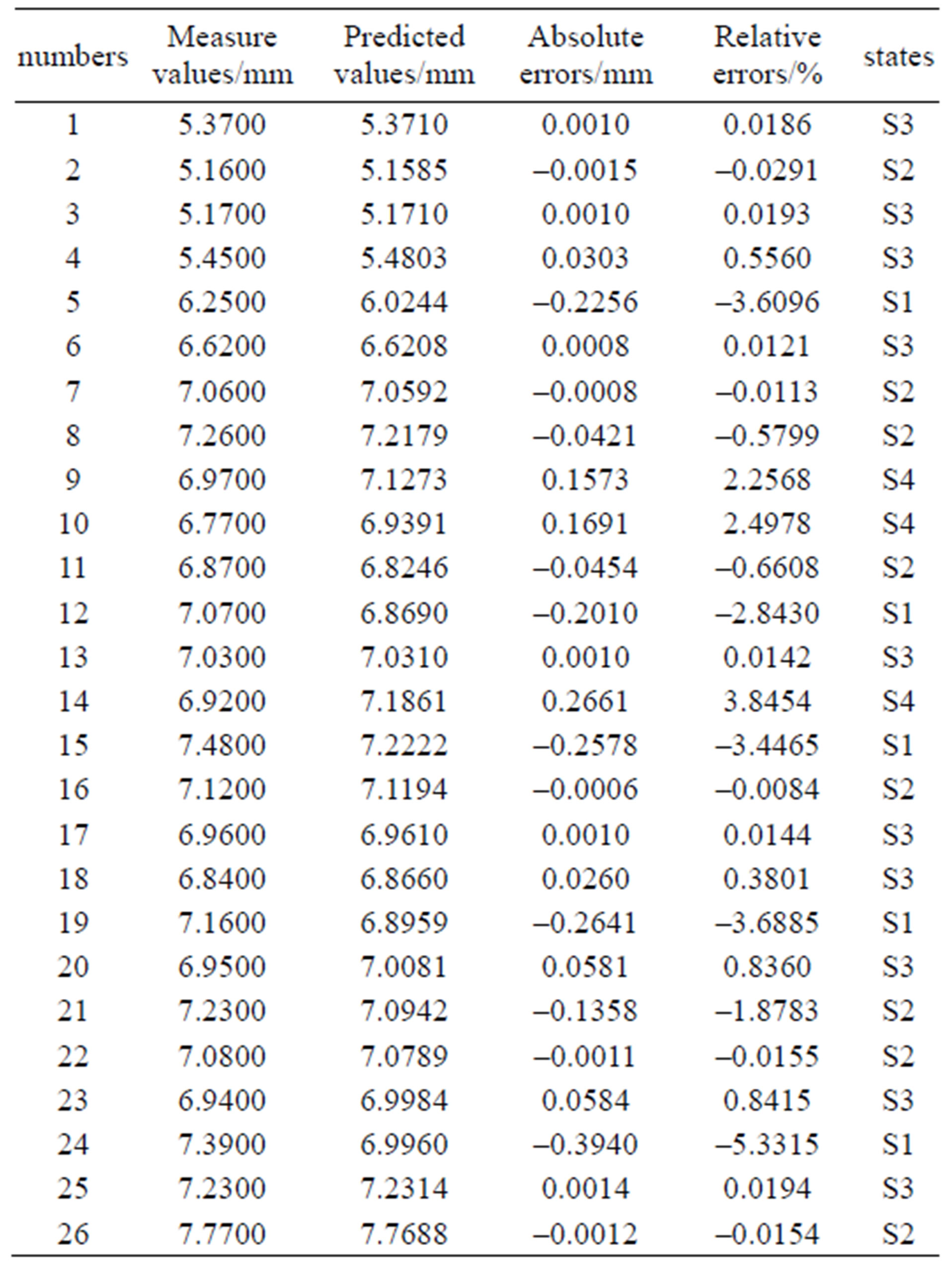
Table 2. Fitted results of 26 initial samples.
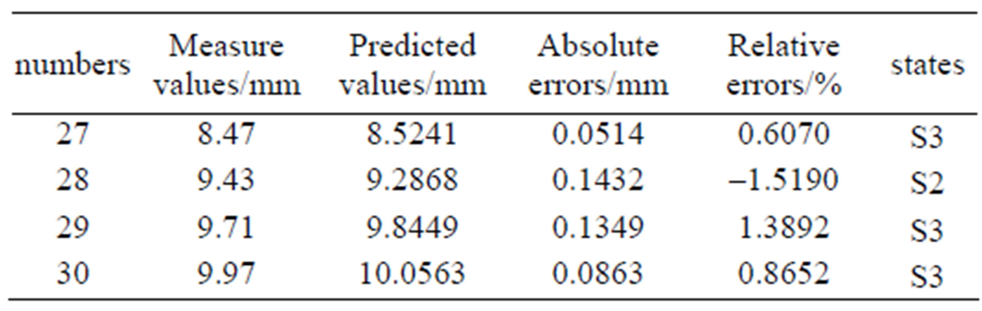
Table 3. GA-LSSVM predicted result of 4 test samples.
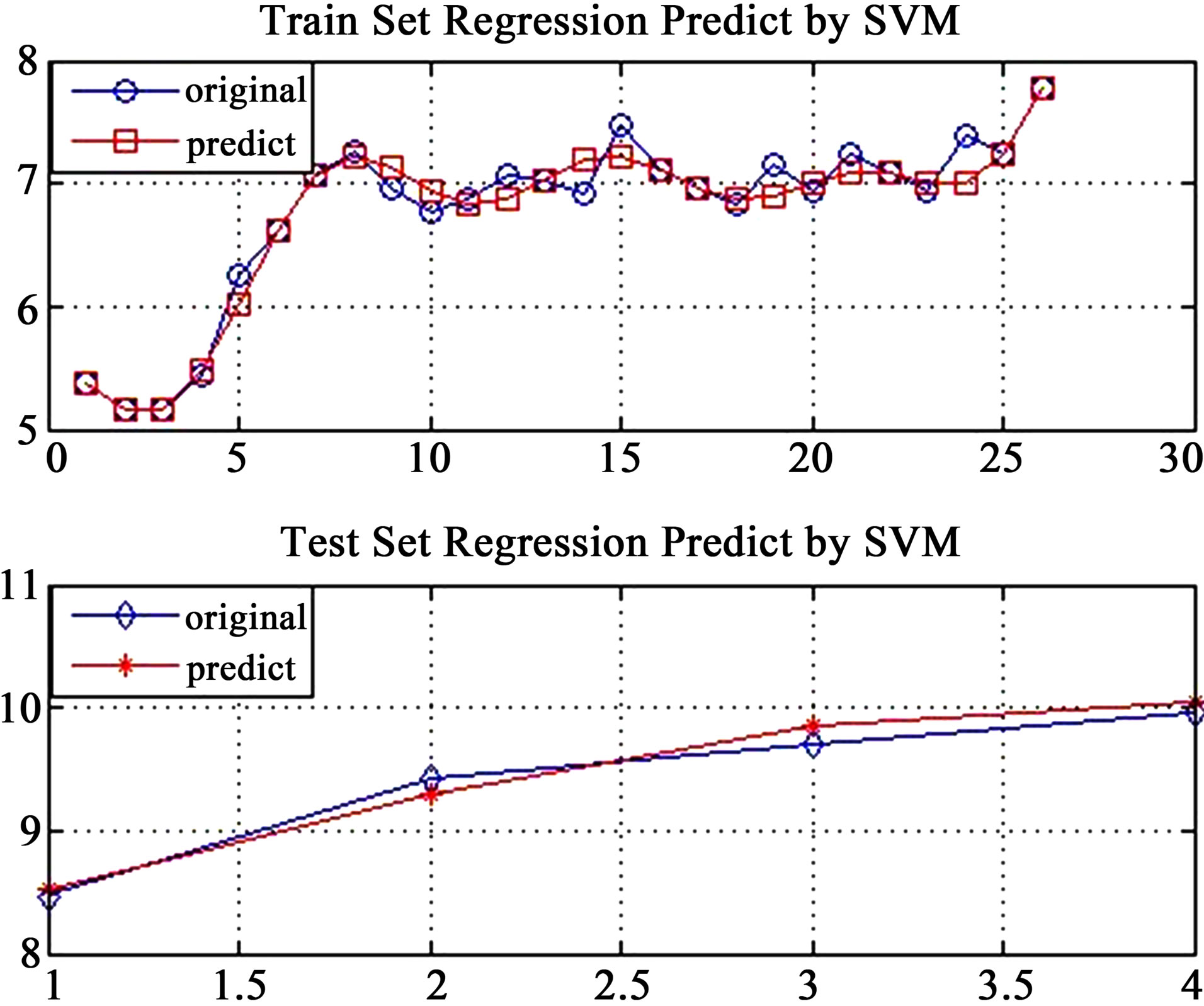
Figure 2. Compared diagram between measured values and predicted values of learning and test samples.
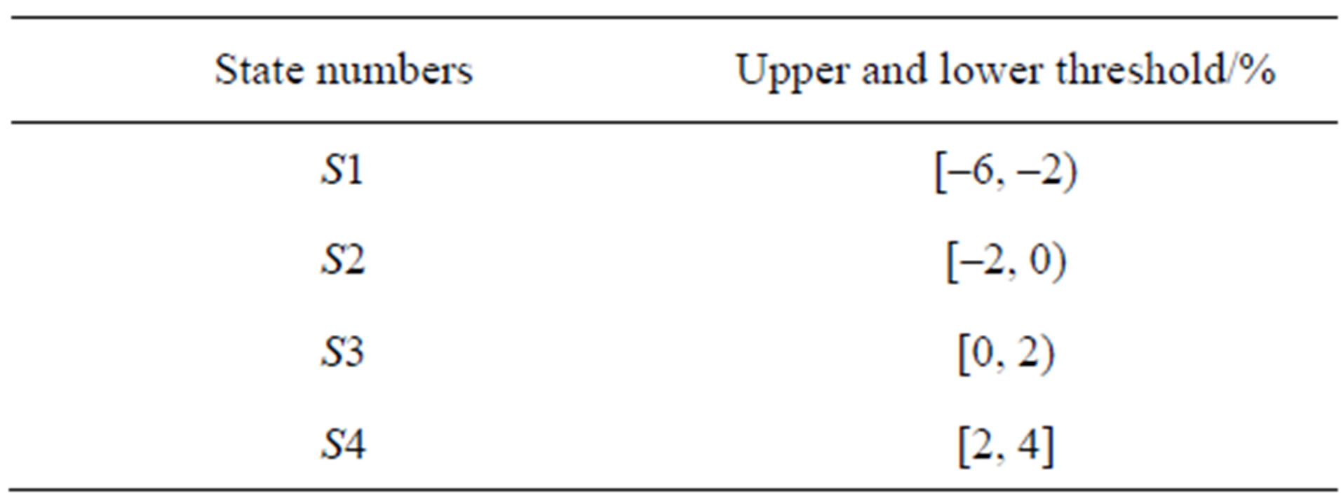
Table 4. State division standard.
3.2.3. The Prediction Table
The state predicts calculation results of step 27 are in Table 5.
According to formulae 3-11 and 3-13, the average relative error value of step 27 is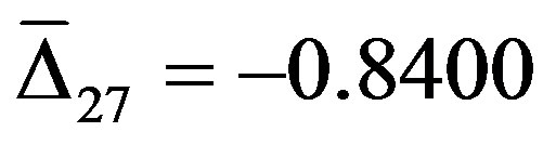 .The prediction value is
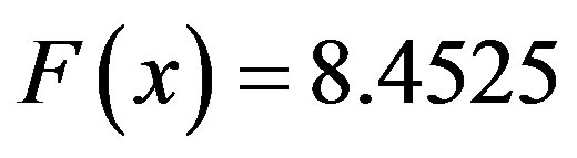 .
.
3.2.4. Dynamic Rolling Prediction
We set dynamic rolling prediction to step 28 to 30, and the calculation results are in Table 6. The accuracy of markov improved prediction model is better than that of LSSVM model in Table 3.
4. CONCLUSIONS
In this paper, LSSVM is improved with GA and markov, and the GA-LSSVM-markov forecast model is built. LSSVM, which can be used to solve problems with little samples, non linear, high dimension and the local minimum points, is used to predict the development rules of surrounding rock deformation. GA, with the advantage that it gets optimal solution through adaptive control search, is used to look for the best input parameters of LSSVM. Markov, which can reflect the micro variation rules of displacement, is used to calculate the transition
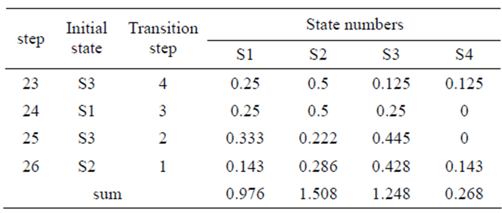
Table 5. The state predict calculation results of step 27.
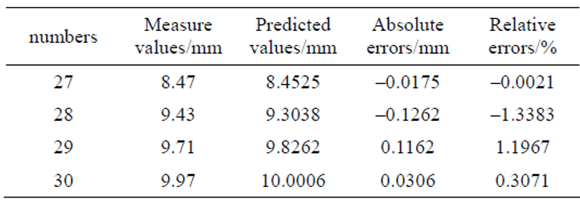
Table 6. The prediction results of GA-LSSVM-markov model.
probability error of LSSVM model, so as to improve the accuracy of prediction model. Been used to certain command protection engineering, the model is proved to be more accurate than obvious models. The model can be spread to other engineering.
REFERENCES
- Guo, W. (2009) Prediction of rock deformation and analysis of rock stability of tunnel based on the neural network. Chongqing University, Chongqing.
- Feng, X.-T. (2000) Intelligent rock mechanics. Science Press, Beijing.
- Zhao, P. (2009) Prediction for surrounding rock deformation of tunnel based on SVM coupling with cyclic variable method. Journal of Shijiazhuang Railway Institute (Natural Science), 22, 61-64.
- Wang, Y.-Y. (2001) Analysis, control and forecast of deformation and pressure in soft rock tunnel. Liaoning Engineering Technology University, Fuxin.
- Wu, Y.-P. and Li, Y.-W. (2008) Application of grey-ENN model to prediction of wall-rock deformation in deep buried tunnels. Rock and Soil Mechanics, 29, 263-266.
- Jiang, Y.-N., Feng, X.-T. and Gao, W. (2002) Study of integration intelligence for constringency displacement analyzing of large cavern group. Chinese Journal of Rock Mechanics and Engineering, 25, 2501-2505.
- Gong, K.-Y. (2004) The application of gray system theory in the roadway tunneling and surrounding rock deformation prediction. Shandong University, Jinan.
- Li, S.-C., Wang, W.-M. and Wang, L.-C. (1997) Application of non linear time series analysis model to displacement forecasting in underground engineering. Chinese Journal of Geotechnical Engineering, 19, 15-20.
- Zhang, Z.-Q., Feng, X.-T. and Yang, C.-X. (1999) Study on applicability of genetic-neural network modeling of nonlinear displacement time series. Rock and Soil Mechanics, 16, 20-24.
- Gao, W. and Zheng, Y.-R. (2003) Back analysis in geotechnical mechanics and its integrated intelligent study. Rock and Soil Mechanics, 37, 114-116.
- Vapnik, V. (1995) The nature of statistical learning theory. Spring Verlag.
- Zhao, H.-B. (2005) Predicting the surrounding deformations of tunnel using support vector machine. Chinese Journal of Rock Mechanics and Engineering, 4, 649-652.
- Thissen, U., Van Brakel, R. and de Weijer, A.P. (2003) Using support vector machines for time series prediction. Chemometrics and Intelligent Laboratory Systems, 69, 35-49. doi:10.1016/S0169-7439(03)00111-4
- Wang, K.-Q., Yang, S.-C. and Dai, T.-H. (2009) Method of optimizing parameter of least squares support vector machines by genetic algorithm. Computer Applications and Software, 26, 649-652.
- Liu, J.-F. and Li, X.-W. (2000) The stochastic process. China Railway Publishing House, Beijing.
- Zhang, F.-M. and Cui, G.-L. (2006) The settlement prediction of foundation pit based on gray markov chain model. Soil Engineering and Foundation, 16, 82-84, 93.
- Xu, F. and Xu, W.-Y. (2010) Prediction of displacement time series based on support vector machines-Markov chain. Rock and Soil Mechanics, 31, 944-948.