Engineering
Vol.5 No.5A(2013), Article ID:31794,8 pages DOI:10.4236/eng.2013.55A001
An Application of Sinc Sum Function in Hilbert Transformer
Department of Electronic Information Engineering, Huaiyin Institute of Technology, Huaian, China
Email: wyljs@sina.com
Copyright © 2013 Yunlong Wang. This is an open access article distributed under the Creative Commons Attribution License, which permits unrestricted use, distribution, and reproduction in any medium, provided the original work is properly cited.
Received January 16, 2013; revised February 18, 2013; accepted February 27, 2013
Keywords: Sinc Sum; Fourier Transform; Hilbert Transformer; FIR Filter
ABSTRACT
An application of the sinc sum function in Hilbert transformer (HT) is studied. The expression of the frequency response of HT is expressed with sinc sum functions. Some properties of sub-amplitude response of HT are proved by using the properties of the sinc sum function. A general HT formula is obtained theoretically and it contains a general window function. As an example three new window functions are obtained. Different from the existing window functions obtained from lowpass filters, these window functions are obtained directly from HT. Comparisons show that new windows are better than the Hanning, Hamming, Blackman and Kaiser windows in terms of HT performances.
1. Introduction
Hilbert transformer (HT) is widely used in engineering, such as damage diagnosis of rotors [1], electroencephalography analysis [2], detection in speech [3], extraction of modal characteristics [4], upmixing stereo signals [5], and vibration analysis [6]. Hilbert-Huang transform is a technique developed in recent years. One of its main parts is HT [4,7]. Reference [8] gives more application examples of HT. About the design method of HT, we can find some methods [9-13], but window method is one of the most frequently used methods [2-4]. The reason is that window method is the simplest one of them and several windows have good performances. The well-known fixed windows are the Hanning, Hamming, Blackman windows and the most frequently used adjustable window is the Kaiser window. These windows are obtained according to the performances of lowpass filters. Consequently, windows with good performances can not easily be obtained because for finding satisfied windows three performances of passband, stopband and transition width of lowpass filters must be given attention to simultaneously. In the study of FIR filter design, a new function is defined as sinc sum function [14] by the author. The function has been used in the design of FIR filters, such as lowpass filters [14] and differentiators [15,16]. Further study shows that it can be used in the design of FIR HT. The definition of the sinc sum function is as follows [14].
For the positive finite integer ![]() and the real independent variable
and the real independent variable![]() , the expression
, the expression
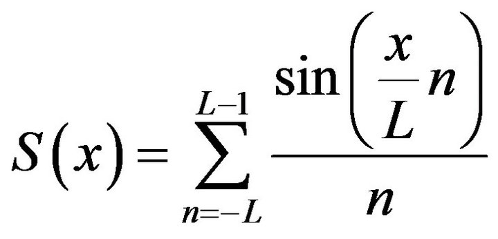 (1)
(1)
is called sinc sum function.
Some properties of the sinc sum function are proved as follows:
(i) Global symmetry:  and
and ;
;
(ii) Stair shape: ;
;
(iii) Local symmetry: 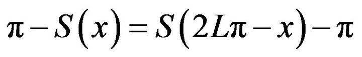 and
and ;
;
(iv) Local extrema certainty: Let
 . Then (a)
  has a local maximum value if
  is an odd number; (b)
  has a local minimum value if k is an even number;
(v) Oscillation regularity: If ![]() increases from 0 to
increases from 0 to , then
  oscillates with decaying magnitude above or below
 ![]() alternatively along with the increase of
alternatively along with the increase of![]() ;
;
(vi) Extreme value stability: Let ![]() be large enough. Then the extreme value and some sub-extreme values of
be large enough. Then the extreme value and some sub-extreme values of  are almost unchangeable along with the change of L.
2. New HT Expression
2.1. Truncated Ideal HT
HT formula in frequency domain is
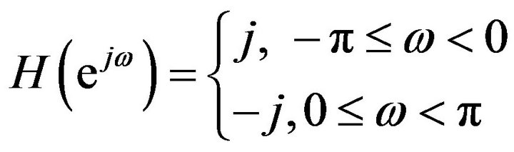 (2)
(2)
Corresponding HT formula in time domain is
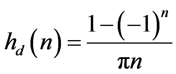 (3)
(3)
We truncate it as follows:
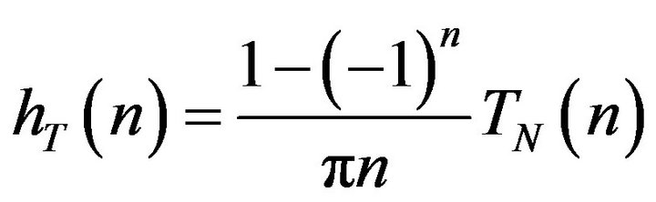 (4)
(4)
where  and
and
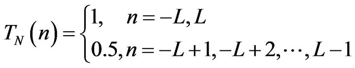 (5)
(5)
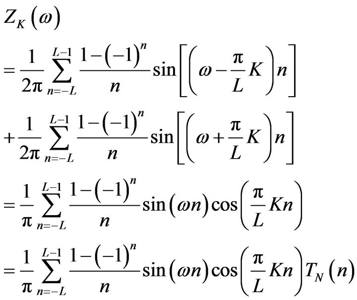
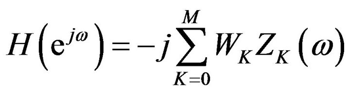
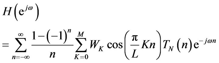
The frequency response of  is
is
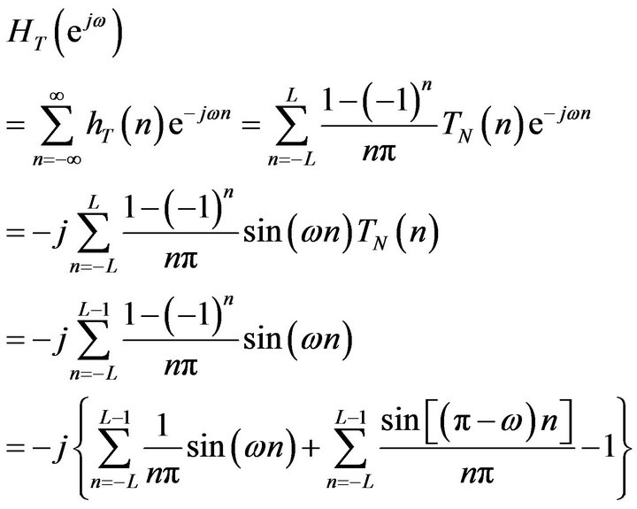 (6)
(6)
In the third step Euler formula is used.
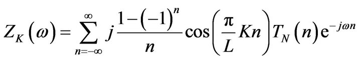
Let . Then it becomes
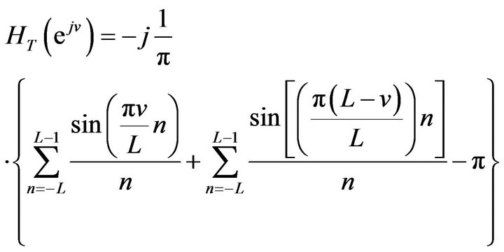 (7)
(7)
This is a new form of frequency response of the truncated HT. Let
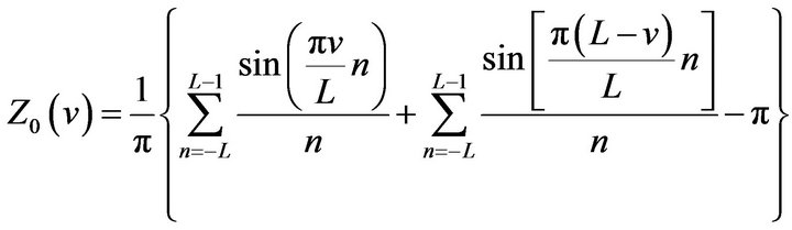
(8)
Theorem 1  of (8) has following properties:
(i)  and
and ;
;
(ii) ;
;
(iii) ;
;
(iv) ;
;
(v)  has a local maximum value if
 ![]() is an odd number and has a local minimum value if
is an odd number and has a local minimum value if ![]() is an even number on the interval
is an even number on the interval ;
;
(vi)  oscillates in the vicinity of 1 on the interval
 .
.
Proof. According to (1), (8) becomes
 (9)
(9)
where  and
and  are two sinc sum functions.
Substituting ![]() for
for ![]() in (9) we get
in (9) we get
 (10)
(10)
By property (ii) of the sinc sum function we get
 (11)
(11)
By property (i) of the sinc sum function we get
 (12)
(12)
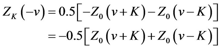
From (2.8) and (2.11) we get
 (13)
(13)
Substituting  in both sides yields
 .
.
Part (i) of the proof is complete.
Substituting  for
for ![]() in (9) we get
in (9) we get
 (14)
(14)
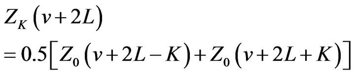
By property (ii) of the sinc sum function and (2.8),
 (15)
(15)
Part (ii) of the proof is complete.
Substituting  for
for ![]() in (9) we get
in (9) we get
 (16)
(16)
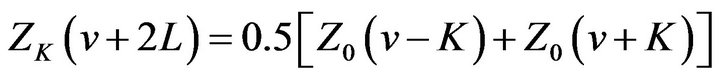
By property (ii) of the sinc sum function we get
 (17)
(17)
By property (i) of the sinc sum function and (2.8),
 (18)
(18)
Part (iii) of the proof is complete.
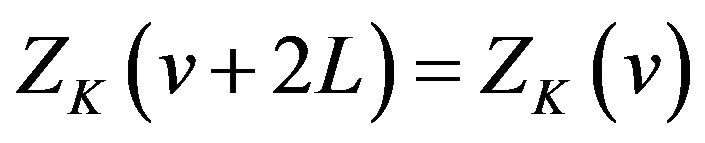
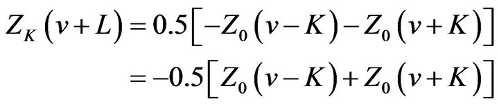
Substituting  for
for ![]() in (9) we immediately get
in (9) we immediately get
 (19)
(19)
Part (iv) of the proof is complete.
By the property (iv) of the sinc sum function,  has a local maximum value if
 ![]() is an odd number and has a local minimum value if
is an odd number and has a local minimum value if ![]() is an even number. The local extreme points of
is an even number. The local extreme points of  relates to the parity of L. For L even,
  and
and  have extrema of the same kind. In this case,
  ,
,  and
and  have extrema of the same kind at any extreme point of
 . For
. For ![]() odd,
odd,  and
and  have extrema of different kinds at each extreme point. But by property (v) of the sinc sum function we always have
  on the interval
 . Then we know that
  and
and
 have extrema of the same kind at any extreme point of
  on the interval. According to (iv) of this theorem the conclusion is still true on the interval
 . Therefore,
  has a local maximum value if
 ![]() is an odd number and has a local minimum value if
is an odd number and has a local minimum value if ![]() is an even number on the interval
is an even number on the interval , no matter how
 ![]() is odd or even.
is odd or even.
Part (v) of the proof is complete.
By property (v) of the sinc sum function,  and
and  are both oscillates in the vicinity of
 ![]() on the interval
on the interval . Then from (9) we easily know that
  oscillates in the vicinity of 1 on the interval.
The proof is complete.
From Theorem 2.1 we can see that  is symmetrical about
 , odd symmetrical about both
  and
and , and periodic with period
 .
.
In addition,  oscillates with decaying amplitude in the vicinity of 1 both from
  to
to  and from
 ![]() to
to . Because the proof is too complexity, we do not prove it in the paper.
2.2. New HT Formula
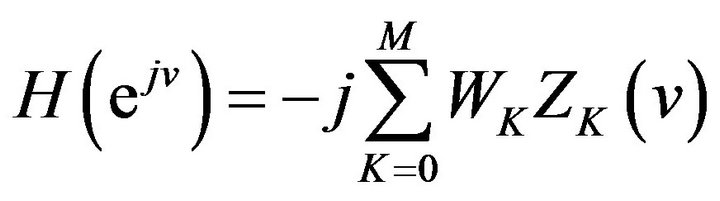
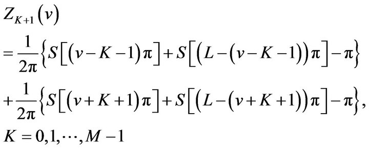
For 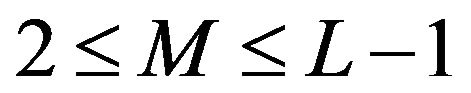 we construct an expression as follows:
 (20)
(20)
where 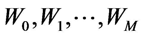 are undetermined weights and
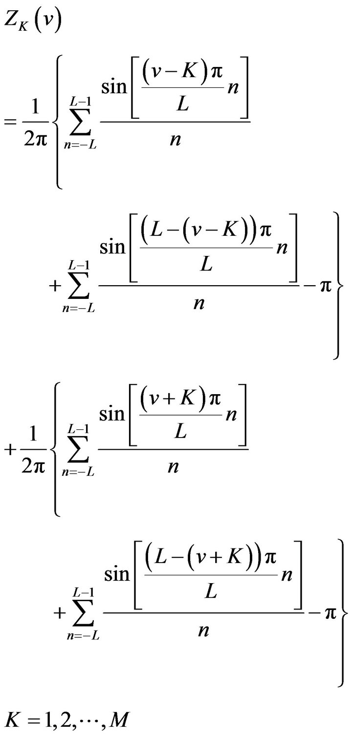 (21)
(21)
Theorem 2  of (21) has following properties:
(i)  and
and ;
;
(ii) ;
;
(iii) ;
;
(iv) ;
;
(v)  has a local maximum value if
  is an odd number and has a local minimum value if
  is an even number on the interval
 ;
;
(vi)  oscillates in the vicinity of 1 on the interval
  and in the vicinity of 0 on both the interval
  and the interval
Proof. According to (1), (21) becomes
 (22)
(22)
where 
and  are four sinc sum functions.
For convenience, let
 (23)
(23)
and
 (24)
(24)
Then (22) becomes
 (25)
(25)
Comparing (23) and (24) with (9), respectively, we get
 (26)
(26)
and
 (27)
(27)
Then (25) becomes
 (28)
(28)
Substituting ![]() for
for ![]() in (28) we get
in (28) we get
By Theorem 2.1 (i) we get
Comparing it with (2.27), we get
 (29)
(29)
Substituting  in both sides yields
 .
.
Part (i) of the proof is complete.
Substituting  for
for ![]() in (28) we get
in (28) we get
By Theorem 2.1 (ii) we get
Comparing it with (2.27), we get
 (30)
(30)
Part (ii) of the proof is complete.
Substituting  for
for ![]() in (28) we get
in (28) we get

By Theorem 2.1 (iii) we get
Comparing it with (2.27), we get
 (31)
(31)
Part (iii) of the proof is complete.
Substituting  for
for ![]() in (28) we get
in (28) we get

By Theorem 2.1 (iv) we get
Comparing it with (2.27), we get
 (32)
(32)
Part (iv) of the proof is complete.
By Theorem 2.1 we know from (26) that  has a local maximum value if
  is an odd number and has a local minimum value if
  is an even number on the interval
 , and we know from (27) that
  has a local maximum value if
  is an odd number and has a local minimum value if
  is an even number on the interval
 . Therefore,
  and
and  have local extrema of the same kind at each extreme point on the interval
 . Then from (25) we know that any common extreme point of
  and
and  is the extreme point of
  on the interval. Thus
  has a local maximum value if
  is an odd number and has a local minimum value if
  is an even number on the interval.
Part (v) of the proof is complete.
By Theorem 2.1 (i) and (v), we know from (26) that  oscillates in the vicinity of 1 on the interval
  and in the vicinity of −1 on the interval
  and that
 ; we know from (27) that
  oscillates in the vicinity of 1 on the interval
  and in the vicinity of −1 on the interval
  and that
 .
.
Then from (2.24) we know that  oscillates in the vicinity of 1 on the interval
  and in the vicinity of 0 on the interval
 . By Theorem 2 (iv) we know that
  oscillates in the vicinity of 0 on the interval
 .
.
The proof is complete.
From Theorem 2.2 we can see that  is symmetrical about
 , odd symmetrical both about
  and about
 , and periodic with period
 .
.
Comparing (2.7) with (2.20), we know that  is a special case of
  with
with . We call each
  sub-amplitude response of HT.
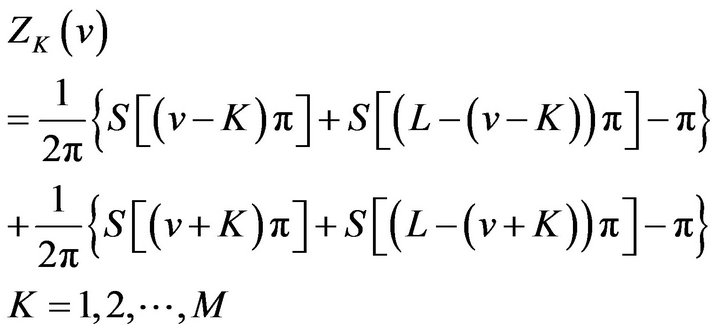
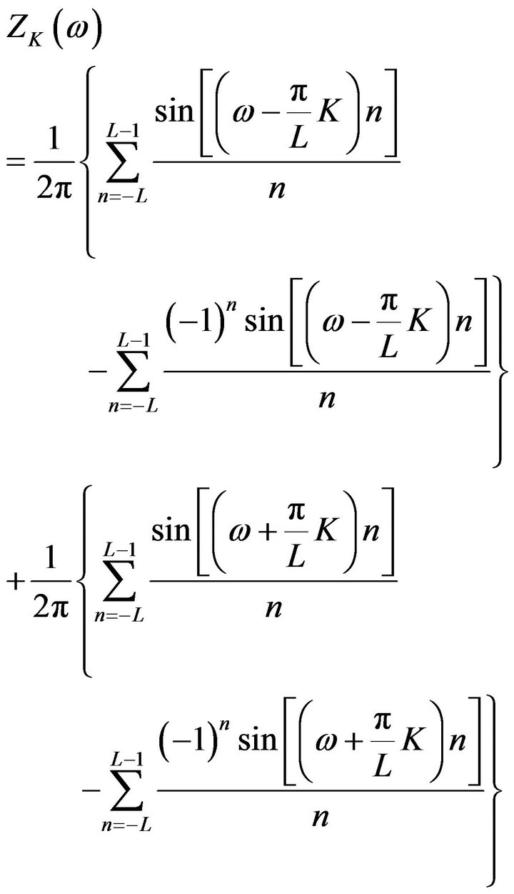
Replacing  by
by  in (2.21), we get
 (33)
(33)
By property (iv) of the sinc sum function, we easily know that  and
and  always have extrema of different kinds at each integer point
 ![]() except
except  and
and  on the interval
 .
.
A plot of  and
and  for
for  are illustrated in Figure 1. We can see that the above analysis is identical with the figure.
By , (21) becomes
 (34)
(34)
Using triangular identity, we have
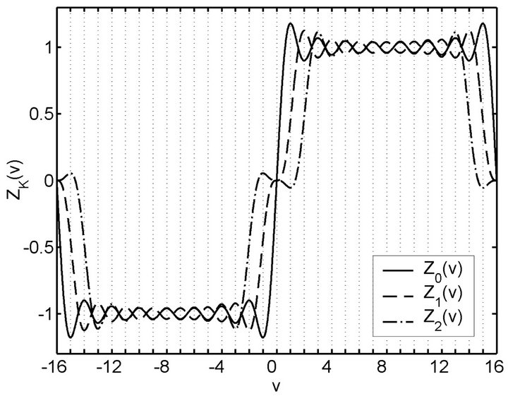
Figure 1.  and
and  for L = 16 on [−16 16].
Using Euler formula, we get
 (35)
(35)
By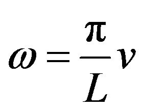 , (2.19) becomes
 (36)
(36)
Substituting (2.34) in (2.35), we get
 (37)
(37)
Corresponding impulse response is
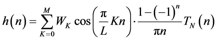 (38)
(38)
or
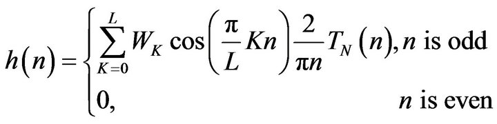 (39)
(39)
From the above discussions about  we can see that if the value of each
  is proper the superposition of all
  can make the maximum deviation of
  decreased because their changes in opposite directions can counteract mostly. Then we can obtain HT formulas with good performances. According to the property (vi) of the sinc sum function,
  is almost unchangeable along with the change of
 ![]() if it is large enough. Thus
if it is large enough. Thus ![]() can be arbitrary under this condition. In general,
can be arbitrary under this condition. In general,  can be considered large enough.
Equation (38) contains a window function as follows:
 (40)
(40)
Now the weight  is the widow constant.
For convenience, let
 (41)
(41)
It is the amplitude of (2.19).
3. Examples of Obtaining HT Formulas
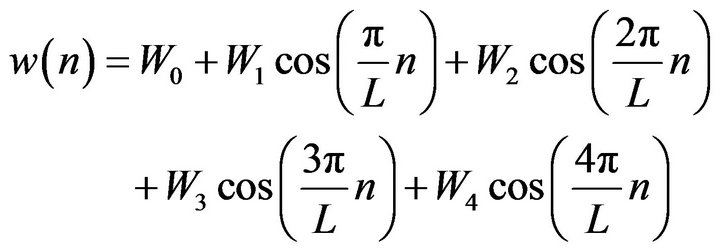
We choose  (correspondingly,
  through 4). Then (41) becomes
 (42)
(42)
We can select 5 points of![]() . In general, it is better to select the local extreme points of
. In general, it is better to select the local extreme points of  denote the 5 points, respectively. Then from (42) we get 5 equations as follows:
 (43)
(43)
 (44)
(44)
 (45)
(45)
 (46)
(46)
 (47)
(47)
Solving the simultaneous equations, we can obtain  through
 .
.
Now we choose , and
, and  as above five points and let
 . Substituting them in (8) and (21), respectively, we get
 ,
,  ,
,  ,
,
 , and
, and , in turn. We do not list theses values here.
 , and
, and  are selected with 3 cases listed in Table 1. They are selected based on the consideration that the resulting windows can easily be compared with the Hanning, Hamming and Blackman windows in terms of HT performances, respectively.
Solving (3.2) we get  through
  listed in table 3.1, too. Then from (39) we obtain HT formula as follows:
 (48)
(48)
Corresponding window is
 (49)
(49)
For , we get corresponding maximum passband ripple of each HT. In Table 1, Ap is the maximum passband ripple and
 ![]() is from the following relationship:
is from the following relationship:
 (50)
(50)
where  is the lower cutoff frequency of magnitude responses.
It is obvious that for finding good window constants we only need to take into account two performances of maximum passband ripple and transition width in the magnitude response of HT.
If maximum passband ripple and lower cutoff frequency as two specifications are known, we can easily design HTs. The first step is to select a window from table 3.1. Then the corresponding ![]() is obtained from the table. The next step is to compute
is obtained from the table. The next step is to compute  according to (50) and further
![]() . The last step is to compute HT coefficients according to (48).
. The last step is to compute HT coefficients according to (48).
4. Compared with Other Windows
Now we compare passband ripples of frequency responses of HTs obtained by using three new windows with those obtained by using the Hanning, Hamming, Blackman and Kaiser windows [17] for , respectively. About the Kaiser window, we select its parameter
  in this way that the maximum passband ripple obtained by using each new window is the same as that obtained by using the Kaiser window. For seeing clearly and reducing paper length we only plot part of each curve in Figure 2. It is necessary to say that for each curve passband ripples oscillate with decaying magnitude
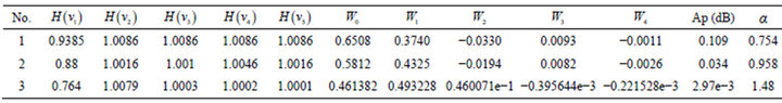
Table 1. Three cases of  through
 ,
,  through
 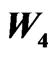 and HT performances.
 (a)
(a)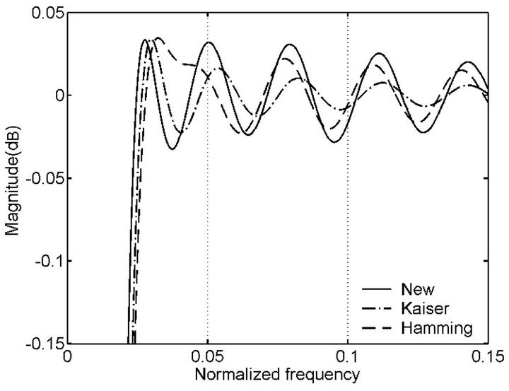 (b)
(b) (c)
(c)
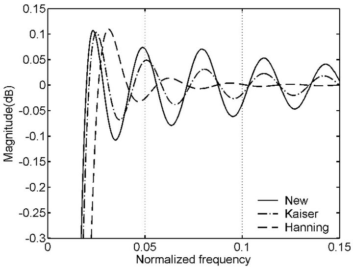
Figure 2. Comparison between new windows with other windows in terms of HT performances for L = 63, respectively. (a) Magnitude response obtained by using new window (No. 1), Kaiser window (β = 3:83) and Hanning window; (b) Magnitude response obtained by using new window (No. 2), Kaiser window (β = 4:98) and Hamming window; (c) Magnitude response obtained by using new window (No. 3), Kaiser window (β = 7:5) and Blackman window.
in the vicinity of 0 dB from some local extrema to the point with the normalized frequency being 0.5 in Figure 2 and the whole curve is symmetrical about the frequency. From the figure we can see that these new windows are better than the Hanning, Hamming, Blackman and Kaiser windows in terms of HT performances, respectively.
5. Conclusion
A general HT formula is deduced by using the sinc sum function and it contains a general window function. Three new windows are obtained directly from the magnitude responses of HT. These new windows belong to fixed window. They are two or three cosine terms more than the Hanning, Hamming and Blackman windows but much simpler than the Kaiser window. Comparisons show that these new windows are better than the Hanning, Hamming, Blackman and Kaiser windows in terms of HT performances.
REFERENCES
- M. Feldman and S. Seibold, “Damage Diagnosis of Rotors: Application of Hilbert Transform and Multihypothesis Testing,” Journal of Vibration and Control, Vol. 5, 1999, pp. 421-442. doi:10.1177/107754639900500305
- W. J. Freeman, “Origin, Structure, and Role of Background EEG Activity. Part 3. Neural Frame Classification,” Clinical Neurophysiology, Vol. 116, No. 5, 2005, pp. 1118-1129. doi:10.1016/j.clinph.2004.12.023
- O. Deshmukh, C. Y. Espy-Wilson, A. Salomon and J. Singh, “Use of Temporal Information: Detection of Periodicity, Aperiodicity, and Pitch in Speech,” IEEE Transactions on Speech Audio Process, Vol. 13, No. 5, 2005, pp. 776-786. doi:10.1109/TSA.2005.851910
- F. L. Zarraga, “On-Line Extraction of Modal Characteristics from Power System Measurements Based on HilbertHuang Analysis,” International Conference on Electrical Engineering, Computing Science and Automatic Control, Toluca, 10-13 January 2009, pp. 1-6.
- C. J. Chun, Y. H. Lee, Y. G. Kim, H. K. Kim and C. S. Cho, “A Real-Time Audio Upmixing Method from Stereo to 7.1-Channel Audio,” Communication and Networking —Communications in Computer and Information Science, Vol. 120, 2010, pp. 162-171.
- F. Michael, “Hilbert Transform in Vibration Analysis,” Mechanical Systems and Signal Processing, Vol. 25, No. 3, 2011, pp. 735-802. doi:10.1016/j.ymssp.2010.07.018
- N. E. Huang, “Introduction to Hilbert-Huang Transform and Its Related Mathematical Problems,” In: N. E. Huang and S. S. P. Shen, Eds., Hilbert-Huang Transform and Its Applications, World Scientific, Singapore City, 2005, pp. 1-26.
- H. Luo, X. Fang and B. Ertas, “Hilbert Transform and Its Engineering Applications,” AIAA Journal, Vol. 47, 2009, pp. 923-932.
- H. W. Schüler and P. Steffen, “Halfband Filters and Hilbert Transformers,” Circuits, Systems and Signal Processing, Vol. 17, No. 2, 1998, pp. 137-164. doi:10.1007/BF01202851
- A. Hossen, “A New Fast Approximate Hilbert Transform with Different Applications,” IIUM Engineering Journal, Vol. 2, No. 2, 2001, pp. 21-27.
- S. W. A. Bergen and A. Antoniou, “Design of Nonrecursive Digital Filters Using the Ultraspherical Window Function,” EURASIP Journal on Applied Signal Processing, Vol. 12, 2005, pp. 1910-1922. doi:10.1155/ASP.2005.1910
- H. Olkkonen, P. Pesola and J. T. Olkkonen, “Computation of Hilbert Transform via Discrete Cosine Transform,” Journal of Signal and Information Processing, Vol. 1, No. 1, 2010, pp. 18-23. doi:10.4236/jsip.2010.11002
- J. T. Olkkonen and H. Olkkonen, “Complex Hilbert Transform Filter,” Journal of Signal and Information Processing, Vol. 2, No. 2, 2011, pp. 112-116. doi:10.4236/jsip.2011.22015
- W. Yunlong, “Sinc Sum Function and Its Application on FIR Filter Design,” Acta Applicandae Mathematicae, Vol. 110, No. 3, 2010, pp. 1037-1056. doi:10.1007/s10440-009-9492-7
- Y. Wang, “An Effective Approach to Finding Differentiator Window Functions Based on Sinc Sum Function,” Circuits, Systems and Signal Processing, Vol. 31, No. 5, 2012, pp. 1809-1828. doi:10.1007/s00034-012-9399-9
- Y. Wang, “New Window Functions for the Design of Narrowband Lowpass Differentiators,” Circuits, Systems and Signal Processing, 2012. doi:10.1007/s00034-012-9536-5
- E. C. Ifeachor and B. W. Jervis, “Digital Signal Processing,” Publishing House of Electronics Industry, Beijing, 2003.