Engineering
Vol. 5 No. 2 (2013) , Article ID: 27727 , 10 pages DOI:10.4236/eng.2013.52023
The Dynamic-to-Static Conversion of Dynamic Fault Trees Using Stochastic Dependency Graphs and Stochastic Activity Networks
1Department of Mathematics and Informatics, University of Catania, Catania, Italy
2Department of Electric, Electronic and Computer Engineering, University of Catania, Catania, Italy
3Department of Drug Sciences, University of Catania, Catania, Italy
Email: gmanno@dmi.unict.it, chiacchio@dmi.unict.it, Francesco.pappalardo@unict.it
Received December 1, 2012; revised January 4, 2013; accepted February 12, 2013
Keywords: Dynamic Fault Tree; Stochastic Dependency Graphs; Stochastic Activity Network; Continuous Time Markov Chain
ABSTRACT
In this paper a new modeling framework for the dependability analysis of complex systems is presented and related to dynamic fault trees (DFTs). The methodology is based on a modular approach: two separate models are used to handle, the fault logic and the stochastic dependencies of the system. Thus, the fault schema, free of any dependency logic, can be easily evaluated, while the dependency schema allows the modeler to design new kind of non-trivial dependencies not easily caught by the traditional holistic methodologies. Moreover, the use of a dependency schema allows building a pure behavioral model that can be used for various kinds of dependability studies. In the paper it is shown how to build and integrate the two modular models and to convert them in a Stochastic Activity Network. Furthermore, based on the construction of the schema that embeds the stochastic dependencies, the procedure to convert DFTs into static fault trees is shown, allowing the resolution of DFTs in a very efficient way.
1. Introduction
Nowadays, technology and technological systems are fundamental constituents of any industrial process. In such a context, the demand of more effective and precise risk assessments and performability evaluations has highlighted the necessity of adequate, specific dependability evaluation techniques and methods. In fact, such dependability techniques and methods have to be able to effectively capture the behavior of modern systems, subsystems and components which could be characterized by interdependencies and interactions. Many methodologies have been formulated to achieve these objectives and implement efficient solution techniques. Among these, Dynamic Fault Tree (DFT) [1,2] stands out for its characteristics including: a valid formalism, a high level language of description and several resolution algorithms. For these reasons DFT has became a benchmark for many other modeling framework for the dependability.
Many efforts have been made to address the following main issues: 1) the problem of the state space explosion of the equivalent Continuous Time Markov Chain (CTMC) [3-7]; and 2) the need of a more generalized formalism to tackle various kind of complex systems and able to perform different dependability studies [8-18]. In [12] a powerful framework able to tackle general dependencies is presented. However, dependencies can be implemented only through connections (i.e., denoted as triggers) between the elements of the Fault Tree. In this way, complex relationships can be added abusing of the Fault Tree notation, which can, in the end, results in an explosion of the tree.
The main motivation of this work is to expand the modeling power capabilities of dependability tools, such as DFTs, and maintain a high level formalism of description. The issues addressed in this paper concern: 1) the lack of the general modeling techniques to include stochastic dependencies between events not directly related by a fault (i.e., a more general approach to model statedependent components behavior); and 2) the handling of general sojourn time distributions, non-Markovian processes (e.g. time delays), inhibitions, multiple failure modes, etc.
To achieve these objectives a modeling framework based on a modular approach is presented. The methodology makes use of two high level models that decouple stochastic dependencies and the system fault logic through:
a stochastic Dependency Graph (DG) and a generic fault schema. Hence, dependability measures are evaluated through the combination of the information provided by these two models.
The framework results incredibly flexible because the DG and the fault schema are independent. The former embeds the dependencies among the components, the latter embeds the system fault logic. Moreover, this last one can be constructed in several ways (i.e. FT, RBD, Event Tree, etc.). In this way, it is possible to generate a behavioral model on the basis of the information contained in the DG and compute many Reward Functions (RF; like the reliability, availability, reliability with repair, conditional probabilities, etc.) attaching the information derived from the system fault schema.
In this paper is presented an application of this modeling framework and a practical case study to convert DFT will be shown: the stochastic dependencies of the DFT will be captured by the DG model, while the system fault logic will be described by a static Fault Tree (FT). In the following this modular model is referred as a Stochastic Dependency Graph Fault Tree (DGFT).
The objectives of this methodology can be listed as follow:
• Create a more flexible approach for the dependability modeling in presence of state-dependent components behavior;
• Model new dependencies logics that are not expressed through the dynamic gates of the DFT;
• Assess various dependability studies using one single model;
• Evaluate dependability measures of complex systems by the mean of analytical and simulating methods easily retrievable from the high level models.
The remainder of the paper is structured as follow: in Section 2 a general description of DGs’ basic elements is given and a general mathematical expression stating the state-dependent transition rate of components with exponential behavior is given; in Section 3 is presented the general procedure to convert DFTs in DGFTs and the subsequent lower level conversion that is needed to calculate the RF; Section 4 is concerned with the derivation of the intermediate level models; in Section 5 a case study (taken from the literature) [10] is solved to show the DFT to DGFT conversion and the resolution procedure; Section 6 reports conclusion and future works.
2. Stochastic Dependency Graphs
A DG is a model that highlights stochastic dependencies between components. The elements of a DG are nodes, direct links and dependency gates. Each component is represented by a node and nodes are linked together by the mean of direct links and dependency gates. Connections represent stochastic relationships among components. Components not affected by stochastic dependencies are drawn as isolated nodes while components subjected to dependencies will be drawn as nodes intercomnected by direct links and gates.
It is worth to distinguish between parents and child components. Parents components are components whose the entering in a particular state force some change in the parameter of the sojourn time distribution (or more generally the entire distribution law) of the child component. A node can be both a parent and a child for some other node.
Among all the kind of dependencies some basic dependency types are reported in this paper: elementary, AND, OR and k/N:
• An elementary dependency exist between a parent and a child component if a change in the state of the parent forces a change in the child sojourn time distribution;
• In an AND dependency gate the child is affected from its parents if all them are in a specific state;
• In an OR dependency gate the child is affected if at least one of its parents is in a specific state;
• In a k/N dependency gate the change is dictated from all the combinations of the N parents where k of them are in a specific state. It generalizes the AND and OR dependency gates in the case that k is respectively equal to N and one. In the case that both k and N are equal to one the dependency gate is further reduced to an elementary dependency link.
Generally the specific state is represented by the failed state. Figure 1 shows the graphical representation of the four kinds of dependencies introduced above.
For a DG constituted by any combination of the basic elements above introduced, qualitative MCS (or DMCS in case of dynamic dependencies) can be derived. They can be used to specify the reactivation conditions in thebehavioral model (see Section 4).
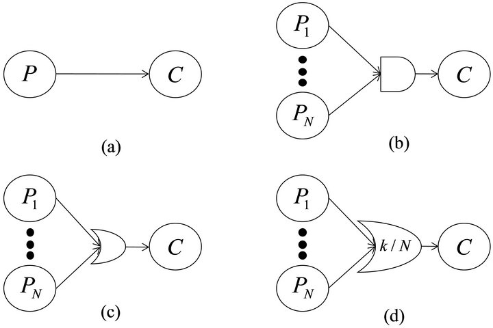
Figure 1. DG elements: (a) Elementary dependency link; (b) AND dependency gate; (c) OR dependency gate; (d) k/N dependency gate. Pi: parent node; C: child node.
In the following a mathematical expression to calculate the system-state-dependent failure rate of a component under a k/N dependency gate is shown. The results refer only to exponential sojourn time distribution but they can be further generalized.
Let us consider a system with two state components (i.e. “working-failed” or “UP-DOWN”). Let us denote with si the state of the generic i-th component: si can assume two values, one or zero standing respectively for working and failed. Let us define the set I as the set of all input component indexes. Let say h as the generic element of I. Thus, .
.
Let call CiI as the set of all the subset of I of cardinality i, with . The cardinality of the generic set CiI is defined as #CiI. Let us denote each subsets of CiI with CiI(j), with
 , #CiI. In this way each subset CiI(j) represents a collection of input indexes. The current failure rate (i.e., dependent on the current parents state configuration) of the child component is given by:
 (1)
(1)
where λnom and  are the failure rate of the child component when: no dependency effects are present (nominal) and when subjected to the dependency effects of the parent f (scaled).
It is necessary to specify that when λnom is equal to zero (e.g. SPARE in cold stand-by or SEQ) the formula 00 is equal to one and that when  is equal to infinite (e.g. FDEP gate) the formula ∞0 is also equal to one (this is not mathematically correct but allows a compact representation of the expression above).
Equation (1) is the most general form to assess the current failure rate of a child component given the state of its parents. It is suitable for each of the dependency gate discussed above.
Equation (1) is enough general to model systems where the failure rate of the child component assumes different values depending on the kind of failed parent (e.g. a repeated component in a SPARE and a FDEP gate). In this case the impact on the failure rate of the child can be different depending on which parent forces the dependency logic. The operator max is used to address situations where the predominant effect must be chosen.
To model some other relationship between parents and child (e.g. modeling joint effects does not require the max operator) other gates can be introduced, thus generalizing the model for any circumstance.
If a DG is composed of a cascade of gates, Equation (1) must be evaluated in a bottom-up procedure. To this end, the possible states of the gates need to be estimated as well as the transition rates determined from these states (Table 1).
3. DFT-DGFT Conversion
In this section the general approach to convert a DFT in a DGFT model is described. The procedure is carried in three steps (Figure 2): the construction of the FT and the DG model (i.e., the high level models); the construction of the behavioral model and the calculation of the MCS (i.e., the medium level models); and the estimation of the RFs.
In the first step the stochastic dependencies included in the logic of SPARE, FDEP and SEQ gates are designed through the DG model. In this way, all the dynamic gates can be replaced by the appropriate static gates (i.e., preserving the fault logic). This is not the case of the PAND gate since no stochastic dependencies are introduced by this gate (i.e., it describes a kind of fault time dependency). A procedure to solve models including this gate is reported in Section 4.
The second step consists in the construction of the medium level models. A model representing the behavior of the system can be constructed on the basis of the DG model. For instance it can be expressed by Generalized Stochastic Petri Nets (GSPN) [14,15,19]. GSPNs are a powerful tool due to the possibility to conduct simulations and convert them in CTMCs. Also more general
Table 1. DG reduction: Ai component name; SAi component state; SAi = 1 “UP; SAi “DOWN”; λi failure rate of child component if parent i is failed.
Figure 2. DFT-DGFT conversion framework.
Discrete Event Simulation (DES) [16-21] models can be used and, in this case, the DG provides a dependency matrix and mathematical expressions (such as (1)) used to update the system-state-dependent distribution law of the system components.
The medium level of the fault model is then extracted in order to evaluate the set of states of the system that concur to the calculation of the RF. This operation is trivial since the FT, obtained at the previous stage, is free of complex formalisms and can be solved via the Minimal Cut Set (MCS) [22]. In some case instead of calculating the MCS, it can be convenient to create the GSPN model of the FT and link it to the GSPN behavioral model. Models concerning with general type of RFs and with fault time dependencies (e.g. PAND gates) can require the construction of this other medium level model.
The RF is finally calculated by joining the two medium level models. The solution can be achieved via the conversion of the GSPN model to a CTMC or obtained via simulation.
Generally, analytical solutions are preferred, but in cases where 1) the state space is too big; 2) the dynamic behavior of the system is too complex; 3) general sojourn time distributions are used, a solution based on simulation can be obtained with precision dependent on the simulating time (i.e., number of batches).
Figure 2 represents schematically the DFT conversion and the resolution process of a DGFT. If the DGFT is used as a stand-alone methodology the procedure starts from the second level of the process depicted in Figure 2. In the case the fault schema used is not a FT, no differences are encountered in the resolution of the model. In fact the MCS represent just that set of condition of interest from a dependability point of view and can be evaluated through any other fault schema.
4. Medium Level Models
Medium level models are used to represent the behavior and the fault logic of the system. The behavioral model is built using the knowledge contained in the DG model. A special class of GSPN—Stochastic Activity Networks (SAN) [19]—were used in this work. Elements of a SAN are: instantaneous and timed activities, input and output gates, places and extended places. A more complete discussion regarding SAN models can be found in [19]. The modeling approach is component based. Each component is represented by a place whose marking specifies its state (e.g. one token “UP”; zero token “DOWN”). For each state a component can assume, an activity representing its shifting among these states must be created. Each activity can be reactivated regarding the change of the marking of the model. To this end, it includes a reactivation predicate that is used to assess if the conditions specified by the DMCS, of the sub-DG of the current modeled component, have changed (i.e., DMCS can be automatically converted in a if statement). Two situations must be distinguished:
• In the case of non-repairable components, the reactivation predicate is based only on the DMCS (Table 1).
• If the system consists of repairable components, apart the DMCS, it must be included all the conditions due to the repair of the parents (Table 2).
Moreover another condition must be added. In fact, the activity can be reactivated only if one of the places representing the parents of the modeled component was the last that changed its marking. These last conditions must be
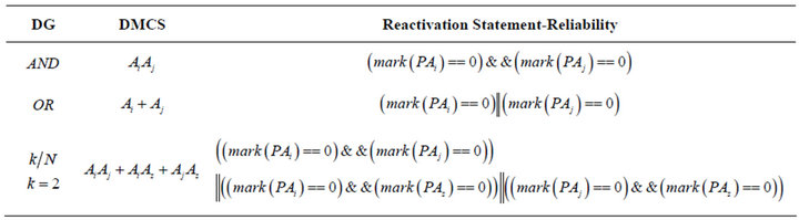
Table 2. DMCS Vs reactivation predicate: reliability. Ai component name; PAi component place; mark (PAi == 1) “UP; mark (PAi == 0) “DOWN”.
added by an and statement to the conditions specified by the DMCS.
Moreover, a distinction must be made in the case the DG is composed of OR and k/N gates. In fact, given the structure of these gates, reactivation occurs each time a component attached to these gates changes its status (OR) or each time a new k condition is reached by the change of some component attached to a k/N gate. Thus we define another statement, the activation predicate. In the SAN language the activation predicate checks if the state when the activity was last activated match the conditions expressed in the statement itself. This is done to avoid reactivation when not wanted, but the modeler could choose to leave the possibility of reactivation just by setting the activation predicate equal to one. The condition to specify in the activation predicate are specified in Table 3.
If a DG is composed of a cascade of gates is possible to evaluate the DMCS following a bottom-up procedure (i.e., from the dependency gates at the lower level to top level).
RFs like the reliability and the availability of the system are calculated by imposing the MCS conditions calculated by the converted static FT. MCS can be attached to the SAN model in the form of an if statement that verifies the marking of the places representing those components concerned in the MCS.
Two issues arise when dealing with reparable components, more specifically when:
1) The goal is to compute the reliability even in presence of repairs (i.e., components can be repaired if the whole system has not failed);
2) If the system has failed, working components cannot longer fail (i.e., the associated CTMC is a truncated CTMC).
In these cases the behavioral model requires information about the state of the whole system. To pass this information, two choices are possible: 1) the construction of a SAN model of the FT; 2) include input gates which disable activities by a statement regarding the occurrence of the MCS.
5. Case Study
In this section an application of the DFT-DGTF conversion is shown. Starting from a DFT the equivalent DGFT is built. Successively, using the information contained in the DG model, a SAN model is implemented using the Mobius® software package, developed from the Center for Reliable and High-Performance Computing at the University of Illinois at Urbana-Champaign [18]. Once the MCS are evaluated from the converted FT they are integrated in the SAN model and used to calculate the reliability of the system.
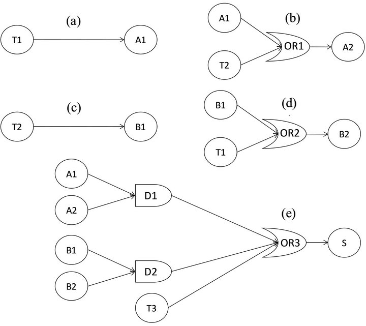
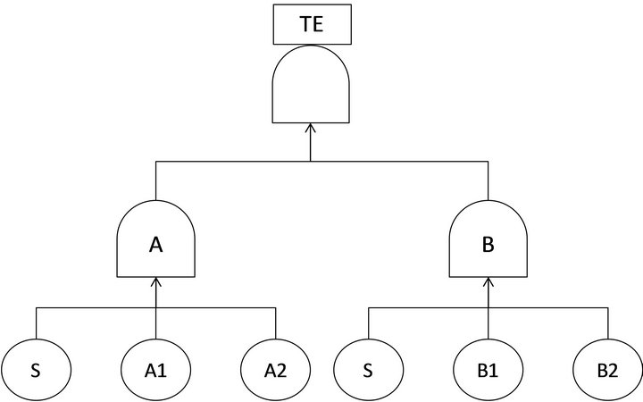
We use a study, from [10], to assess the potentiality of the DGFT methodology due to the presence of repeated events shared among different dynamic gates. All the components are non-repairable characterized by a time to failure exponentially distributed. The DFT of the case study is shown in Figure 3. Its elements are: the basic events A1, A2, B1, B2, S, T1, T2, T3; the gates A (SPARE gate with an active component: A1; and two spares: A2, S), B (SPARE gate with an active component: B1; and two spares: B2, S), F1 (FDEP gate with trigger T1 and components A1 and B2), F2 (FDEP gate with trigger T2 and components A1 and B2), F3 (FDEP gate with trigger T3 and component S), TE (AND gate with gates A, B, F1, F2, F3 as inputs).
5.1. DG Construction
The Construction of the DG of the system requires finding the parents of each component. All the components are attached to dynamic gates, thus, no isolated nodes are present in the DG (Figure 4). The model is retrieved using the procedure stated in Section 4 to convert DFT gates. OR gates are used to model dependencies among different dynamic gates.
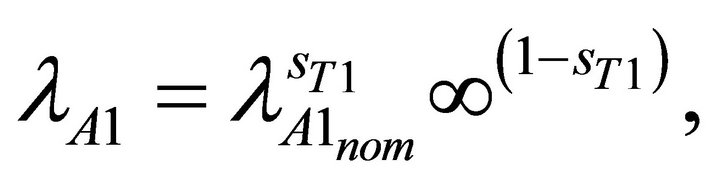
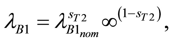
A1 and B1 are subject to the dependency effect of T1 and T2. The DG for these two components is then composed of an elementary dependency link.
Using Equation (1), the mathematical expressions of the state-dependent failure rates of the child components are derived. They are:
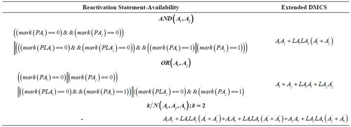
Table 3. DMCS Vs reactivation predicate: availability. Ai component name; PAi component place; mark (PAi == 1) “UP; mark (PAi == 0) “DOWN”;  a check on the inverse condition must be made; LAi, PLAi are used to represent the past state of Ai.
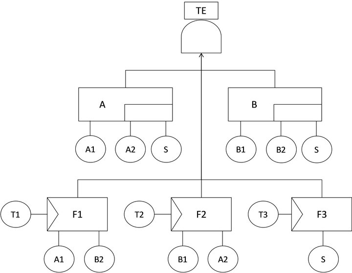
Figure 3. DFT-DGFT conversion framework.
 (2)
(2)
 (3)
(3)
where  and
and  are the nominal failure rates of the two modeled components (when no affected by any dependency effect). sT1 and sT2 represent the state of the trigger events (i.e., 0 if failed, 1 if not).
The DG of A2 and B2, is represented by an OR dependency gate with two inputs: the first one represents the active component of the SPARE and the other the trigger event of the FDEP of the gates they respectively belong to. The simplified expressions of the state-dependent failure rates of A2 and B2 are:
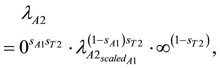 (4)
(4)
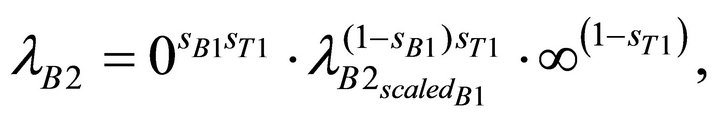 (5)
(5)
where  and
and  are the failure rates of A2 and B2 when operating. sA1, sA2 sT1 and sT2 represent the state of the parent components.
Finally component S is modeled by an OR dependency gate holding three inputs which stand for: the case the S is required from the SPARE A, from the SPARE B and the case the trigger T3 occurs. The DG model that embeds the dependencies of the components A1/A2 (or B1/B2) on S through the SPARE are represented by an AND dependency gate, since S is a spare component of the second order (i.e., positioned as a second spare component in each gate). The simplified expression of the state-dependent failure rate of S is:
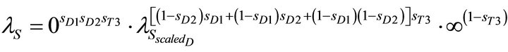 (6)
(6)
where 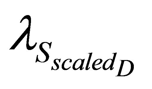 is the failure rate of S when operating as substituting components (i.e., the dependency effect is the same under D1 and D2). In this case a bottom-up procedure to retrieve the state-dependent failure rates was used. Thus sD1, sD2, represent the state of the gates D1 and D2 and sT3 the state of the trigger T3. More specifically
 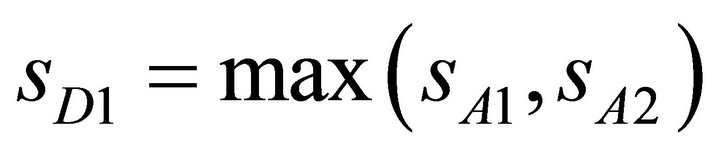 and
and 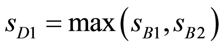 with sA2, sB2 respectively the state of A2 and B2.
5.2. FT Construction
The static representation of the DFT in Figure 3 is shown in Figure 5. In this pure fault logic model FDEP gates are no longer present.
The model results simplified in a top level gate, the AND of the previous model, that holds two more AND gates (A and B) with three inputs for each. The two AND gates result from the conversion of the two SPARE gates of the DFT model. In the general case they should be two k/N gates but, since the number of active components is equal to one, the rule of Section 4 states that k is equal to N. Thus the gates result simplified in two AND gates.
5.3. Medium Levels Models Construction
Avoid In the SAN behavioral model each component is modeled by the following elements:
• PX; place that represent the state of the component X (i.e., mark (PX) = 1 if UP; o if DOWN). In the following with X it is denoted any of the components A1, A2, B1, B2, S, T1, T2, T3.
• Failure activity: timed activity that represents the failure of the component. In the failure activity are specified the failure rate of the component and the reactivation predicate.
• For the sake of clarity it is needed to specify that the notation sX, representing the state of the component X in any of the Equation from (2) - (6), is substituted with the notation mark (PX).
• The reactivation predicate is specified by combining a statement with two sets of conditions: 1) the one arising from the last component that experienced a transition (Table 4); and 2) the one arising from the DMCS of the DG associated with the component X (Table 5).
• An output gate used to store in the place ID the identifier number of the component when the related activity fires.
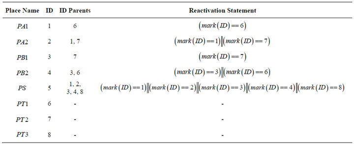
Table 4. Additional condition in the reactivation predicate: in place ID is stored the identifier number of the last componentplace that changed its marking.
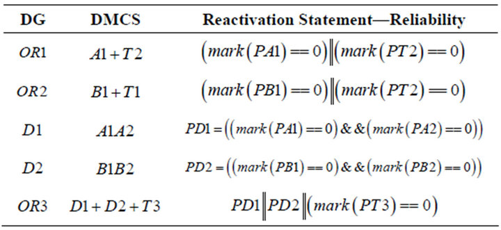
Table 5. DMCS Vs reactivation predicate: reliability. Mark (PX(i) = 0), “DOWN”; mark (PX(i) = 1), “UP”.
• ID; place, shared between all the components, where is stored the identifier number of the last componentplace that changed its marking.
• The model of a generic component in a SAN model is shown in Figure 6.
The MCS of the FT in Figure 5 is:
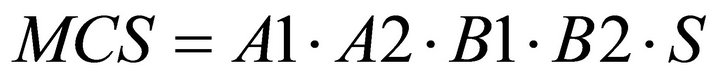 (7)
(7)
This information is used when defining the RF. In this case a check on the marking of the places PA1, PA2, PB1, PB2 and PS of the SAN behavioral model is made at the time the RF is willed to be evaluated.
5.4. Evaluation of the RF: Reliability
The goal of the present case study is to evaluate the reliability of the system modeled by the DFT in Figure 3. The time to failure of all components is exponentially distributed and the failure rate values can be found in Table 6. From reference [10] the reliability value of the system at 100 time units is 0.03126.
The model was resolved analytically (i.e., converting the SAN model in a CTMC) and via simulation. When converted to the low level model the Mobius® Transformer found 256 states (reduced to 48 in the solving phase). The absorbing states were found to be 8. The
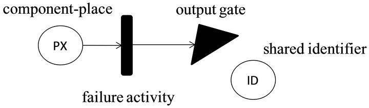
Figure 6. SAN model of a generic component.
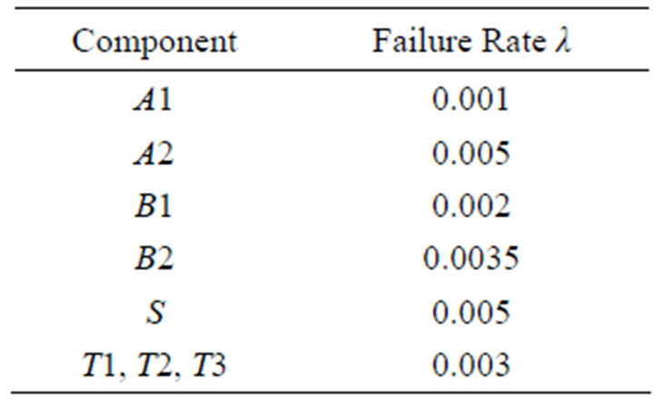
Table 6. Components failure rate [time unit-1].
reliability value was equal to 3.126453e-002 confirming the result in [10].
The Simulator results are reported in Table 7. Again, the results found in [10] are matched. The experiment was carried out by a laptop with the following characteristics: CPU, Intel Core 2 Duo 1.83 GHz; RAM, 1.99 GB.
6. Conclusions
This paper introduces a new modeling framework for the dependability assessment of complex stochastic systems. DGFT is a high level modeling methodology easy to use, intuitive and computationally efficient based on two separated system models: the Stochastic Dependency Graph and a generic fault schema.
DGs allow to exploit many kinds of stochastic dependencies that are not easily caught by other methodologies. The fault schema of the system results simplified from complex relations and can be easily solved. More-
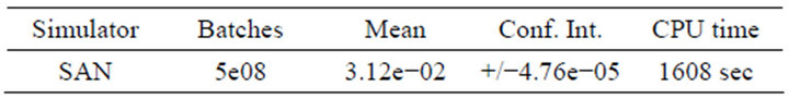
Table 7. Simulator solver results.
over DGs can be converted efficiently in their related behavioral model. Furthermore the behavioral model, being free of any fault logic, results a very flexible mean to conduct various dependability studies.
The main advantages of DGFT are, thus, 1) the possibility of building high-level-high-descriptive models very close to the real structure of the system; 2) the effectiveness of tackling state-dependent component behaviors; 3) and its convertibility in effective and capable lower level models that can be easily improved and modified and that make easier the task of estimating dependability measures, perform sensitivity and uncertainty analysis, diagnosis and other assessments.
DGFT can be used as a stand-alone methodology or as a starting point to build SAN models of dependable systems. Moreover, by this methodology, it is possible to solve efficiently DFTs by converting them to their related FT model.
Future works may go towards: 1) the formalization of a general theory regarding Stochastic Dependency Graphs and their implication in terms of behavioral models; 2) the integration of more advanced tools to resolve fault time dependencies (e.g. dependencies introduced by PAND gates); and 3) the DGFT automatic conversion in SAN models which have shown their potentiality to solve complex dependable systems, both analytically and via simulation, and thus, allowing to model and solve a very general class of complex systems.
REFERENCES
- J. B. Dugan and S. J. Bavuso, “Fault Trees and Sequence Dependencies,” Proceedings of Annual Reliability and Maintainability Symposium, Los Angeles, 23-25 January 1990, pp. 232-235. doi:10.1109/ARMS.1990.67971
- J. B. Dugan and S. J. Bavuso, “Dynamic Fault-Tree Models for Fault Tolerant Computer Systems,” IEEE Transactions on Reliability, Vol. 41, No. 3, 1992, pp. 363-377. doi:10.1109/24.159800
- S. Amari, G. Dill and E. Howald, “A New Approach to Solve Dynamic Fault Trees,” Annual Reliability and Maintainability Symposium, 2003, pp. 374-379.
- R. Gulati and J. B. Dugan, “A Modular Approach for Analyzing Static and Dynamic Fault Trees,” Proceedings of Annual Reliability and Maintainability Symposium, Philadelphia, 13-16 January 1997, pp. 57-63. doi:10.1109/RAMS.1997.571665
- M. Lanus, L. Yin and K. S. Trivedi, “Hierarchical Composition and Aggregation of State-Based Availability and Performability Models,” IEEE Transactions on Reliability, Vol. 52, No. 1, 2003, pp. 44-52. doi:10.1109/TR.2002.805781
- B. N. Feinberg and S. S. Chiu, “A Method to Calculate Steady-State Distributions of Large Markov Chains by Aggregating States,” Operations Research, Vol. 35, No. 2, 1987, pp. 282-290. doi:10.1287/opre.35.2.282
- M. Malhotra and K. S. Trivedi, “A Methodology for Formal Specification of Hierarchy in Model Solution,” Proceedings of 5th International Workshop Petri Nets and Performance Models, (PNPM-1993), Toulouse, 19- 22 October 1999, pp. 258-267. doi:10.1109/PNPM.1993.393445
- S. Distefano and A. Puliafito, “Dynamic Reliability Block Diagrams vs Dynamic Fault Trees,” Proceedings of Annual Reliability and Maintainability Symposium RAMS’07, Orlando, 22-25 January 2007, pp. 71-76.
- A. Bobbio, L. Portinale, M. Minichino and E. Ciancamerla, “Improving the Analysis of Dependable Systems by Mapping Fault Trees into Bayesian Networks,” Reliability Engineering and System Safety, Vol. 71, No. 3, 2001, pp. 249-260. doi:10.1016/S0951-8320(00)00077-6
- H. Boudali and J. Dugan, “A New Bayesian Network Approach to Solve Dynamic Fault Trees,” Proceedings of Annual Reliability and Maintainability Symposium, Alexandria, 24-27 January 2005, pp. 451-456. doi:10.1109/RAMS.2005.1408404
- H. Boudali and J. B. Dugan, “A Continuous-Time Bayesian Network Reliability Modeling, and Analysis Framework,” IEEE Transactions on Reliability, Vol. 55, No. 1, 2006, pp. 86-97. doi:10.1109/TR.2005.859228
- M. Bouissou and J. L. Bon, “A New Formalism That Combines Advantages of Fault-Trees and Markov Models: Boolean Logic Driven Markov Processes,” Relibility Engineering and System Safety, Vol. 82, No. 2, 2003, pp. 149-163. doi:10.1016/S0951-8320(03)00143-1
- S. Swaminathan and C. Smidts, “The Event Sequence Diagram Framework for Dynamic Probabilistic Risk Assessment,” Reliability Engineering and System Safety, Vol. 63, No. 1, 1999, pp. 73-90. doi:10.1016/S0951-8320(98)00027-1
- D. Codetta-Raiteri, “The Conversion of Dynamic Fault Trees to Stochastic Petri Nets, as a case of Graph Transformation,” Electronic Notes in Electronic Computer Science, 127, No. 2, 2005, pp. 45-60. doi:10.1016/j.entcs.2005.02.005
- V. Volovoi, “Modeling of System Reliability Petri Nets with Aging Tokens,” Reliability Engineering and System Safety, Vol. 84, No. 2, 2004, pp. 149-161. doi:10.1016/j.ress.2003.10.013
- M. Marsaguerra, E. Zio, J. Devooght and P. E. Labeau, “A Concept Paper on dynamic Reliability via Monte Carlo Simulation,” Mathematics and Computers in Simulation, Vol. 47, No. 2-5, 1998, pp. 371-382. doi:10.1016/S0378-4754(98)00112-8
- E. Zio, M. Marella and L. Podollini, “A Monte Carlo Simulation Approach to the Availability Assessment of Multi-State Systems with Operational Dependencies,” Reliability Engineering and System Safety, Vol. 92, No. 7, 2007, pp. 871-882. doi:10.1016/j.ress.2006.04.024
- Mobius. http://www.mobius.illinois.edu/
- W. H. Sanders and J. F. Meyer, “Stochastic Activity Networks: Formal Definitions and Concepts,” In: H. Hermanns and J.-P. Katoen, Eds., Lectures on Formal Methods and Performance Analysis, Springer Verlag, Berlin, 2002, pp. 315-343.
- F. Chiacchio, D. D’Urso, N. Trapani, G. Manno and L. Compagno, “Dynamic Fault Trees Resolution: A Conscious Trade-Off between Analytical and Simulative Approaches,” Reliability Engineering and System Safety, Vol. 96, No. 11, 2011, pp. 1115-1126. doi:10.1016/j.ress.2011.06.014
- G. Manno, F. Chiacchio, L. Compagno, D. D’Urso and N. Trapani, “Matcarlore: An Integrated FT and Monte Carlo Simulink Tool for the Reliability Assessment of Dynamic Fault Tree,” Expert Systems with Applications, Vol. 39, No. 12, 2012, pp. 10334-10342. doi:10.1016/j.eswa.2011.12.020
- A. Rauzy, “Binary Decision Diagrams for Reliability Studies,” Handook of Performability Engineering, 2008, pp. 381-339.