Engineering
Vol. 4 No. 3 (2012) , Article ID: 18328 , 6 pages DOI:10.4236/eng.2012.43017
Unsteady Spillway Flows by Singular Integral Operators Method
Interpaper Research Organization, Athens, Greece
Email: eladopoulos@interpaper.org
Received November 15, 2011; revised December 15, 2011; accepted December 25, 2011
Keywords: Unsteady Flows; Spillway; Free-Surface; Open Channel Hydraulics; Singular Integral Operators Method (S.I.O.M.); Constant & Linear Elements; Potential Flows
ABSTRACT
The Singular Integral Operators Method (S.I.O.M.) is applied to the determination of the free-surface profile of an unsteady flow over a spillway, which defines a classical hydraulics problem in open channel flow. Thus, with a known flow rate Q, then the velocities and the elevations are computed on the free surface of the spillway flow. For the numerical evaluation of the singular integral equations both constant and linear elements are used. An application is finally given to the determination of the free-surface profile of a special spillway and comparing the numerical results with corresponding results by the Boundary Integral Equation Method (B.I.E.M.) and by using experiments.
1. Introduction
Gravity driven free-surface flows, belonging to a major field of classical hydraulics problems, were not solved accurately and efficiently in the past, because of several design and measurement purposes. The difficulty for solving such hydrodynamics problems is due not only because of the nonlinear character of the boundary conditions, but from the fact that the boundary of the freesurface flow is not known from the beginning, as well.
Generally the spillway solutions are considerably more difficult to be determined than of the corresponding usual free-surface hydraulics problems, in open channel flow. The basic parameters of the spillway flows, such as discharge, free surfaces and speeds are very important for the design of the hydraulic structures. Over the past years the above parameters were mainly obtained through experiments. On the other hand, the rapid development of computer techniques in hydraulics problems during the recent years, made efficient the possibility to obtain such data by using numerical techniques.
As a beginning, R. V. Southwell and G. Vaisey [1] used finite differences for the investigation of the free waterfall. The finite difference method was further successfully applied by J. S. Mc Nown, E. Y. Hsu & C. S. Yih [2] and by J. J. Cassidy [3] for the calculation of the flow over a spillway.
Furthermore, the study of hydraulics problems by using finite elements, was as a start proposed by J. A. Mc Corquodale and C. Y. Li [4], by investigating sluice gate flows. The finite element method was further applied by S. T. K. Chan, B. E. Larock and L. R. Hermann [5] for the solution of the surface fluid flows and M. Ikegawa and K. Washizu [6] for the investigation of a flow over a spillway crest.
In addition the finite element method was improved by L. T. Isaacs [7,8] for solving potential flow problems and sluice gate flows. Also by using finite elements B. E. Larock [9] studied spillway flows and H.J. Diersch, A. Schirmer and K. F. Bush [10] investigated several generalized hydraulics problems. At the same time E. Varoglou and W. D. L. Finn [11] and P. L. Betts [12] applied the finite element method for the solution of free surface gravity flows.
On the other hand, several open channel hydraulics problems and especially those involved to the determination of a free surface under non-linear boundary conditions were solved by J. A. Ligget [13] and A. H.-D. Cheng, J. A. Liggett and P. L.-F. Liu [14] by using the Boundary Element Method (B.E.M.).
The complex variable function theory was further used for the solution of free surface potential flow problems. This method was applied in the specific cases where the geometry of the solid boundary consists of straight segments and the effort of gravity is neglected. T.S. Strelkoff [15] used a numerical method based on the complex variable function theory for the computation of the sharpcrested weir flows. By using a corresponding method T. S. Strelkoff and M. S. Moayeri [16] studied the waterfall from a flat channel with horizontal and vertical walls. Furthermore, Y. Guo et al. [17] proposed a numerical method for the determination of the spillway flow with free drop an initially unknown discharge.
Over the past years E.G. Ladopoulos [18-26] and E.G. Ladopoulos et al. [27,28] introduced and investigated linear and non-linear singular integral equation methods for the solution of fluid mechanics problems. In the present research the above methods will be extended to the solution of potential and unsteady flows problems over spillways. Thus, the Singular Integral Operators Method (S.I.O.M.) [23-38] is applied to the determination of the free-surface profile of a spillway. For the numerical evaluation of the singular integral equations both constant and linear elements are used. An application is finally given to the determination of the free-surface profile of a spillway and comparing the outprints with corresponding results by the Boundary Integral Equation Method (B.I.E.M.) and by using experiments.
The S.I.O.M. offers many advantages over the B.I.E.M. or Boundary Element Method (B.E.M.), as uses very specific algorithms and code written in Visual Basic in order to run faster and much more accurately.
Whenever the S.I.O.M. was compared to the B.I.E.M. for the solution of problems where closed form solutions were available, then the S.I.O.M. gave solutions much more close to the exact solutions.
2. Basic Formulation for Potential Flow Problems
Consider a homogeneous, incompressible and inviscid fluid, which flows over a spillway. As the flow is irrotational, then for the stream function f, with , is valid [26]:
 (2.1)
(2.1)
Furthermore, because of the conservation of mass for an incompressible fluid, then one has:
 (2.2)
(2.2)
By using (2.1) and (2.2.) we obtain the equation of Laplace which is the governing equation in the domain Ω:
 (2.3)
(2.3)
The boundary conditions corresponding to this problem are:
1) Essential conditions of the type: f = 0 on the lower boundary and on the spillway wall and f = Q on the free surface (2.4)
where Q denotes the flow rate per unit width.
2) Natural conditions of the following type:
 (2.5)
(2.5)
in which v is the velocity and n the unit normal from the free surface.
Furthermore, on the free surface the dynamic boundary condition is valid:
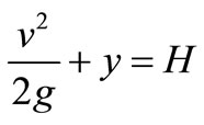 (2.6)
(2.6)
where g is the acceleration of gravity, y the free surface elevation and H the design load (see Figure 1).
Thus, because of (2.6) the natural condition (2.5) takes the form:
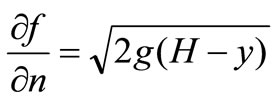 (2.7)
(2.7)
In the current problem of the flow over a spillway, the flow rate Q is known, while the design load H is required as part of the solution. When the flow rate Q is changed per time, then the flow becomes unsteady. In this case the behavior of the flow over the spillway becomes more complicated.
The spillway flow extend to ±¥, but for the purposes of the numerical solution the inflow and outflow streams are cut at right angles to the primary velocity. Hence, on the cut portions the following boundary condition is valid:
 (2.8)
(2.8)
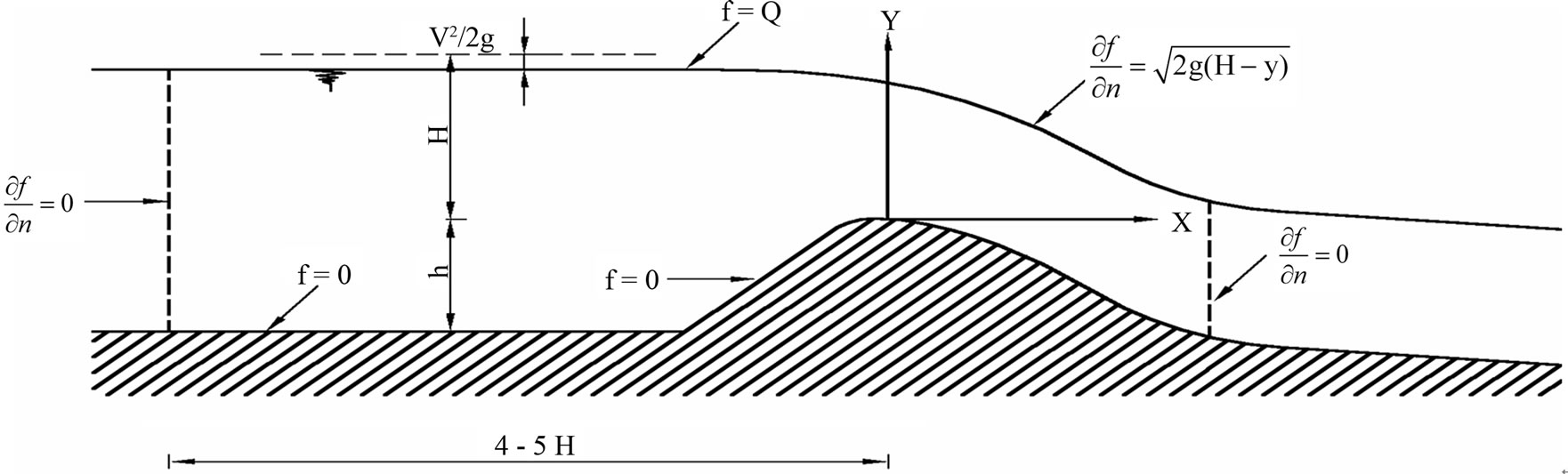
Figure 1. Free-surface profile of a spillway.
By condition (2.8) follows that there is no velocity normal to the main flow. Although this condition is approximate, it is applied enough far from the spillway crest and thus any small error does not affect the interesting part of the flow.
So, with a known flow rate Q, the position of the free-surface boundary is assumed and then the problem is solved by using the above described boundary conditions. Then, by Equation (2.6) the hydraulic load H is calculated on the free surface. Thus, if H is the same for all free-surface points, then the problem is solved. Otherwise, the assumed free surface is changed, so that the hydraulic load H becomes constant at all points.
3. Potential Flow Analysis by the Singular Integral Operators Method
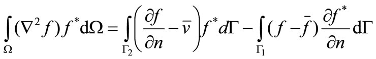
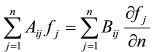
A weighting function f* is introduced, so that it has continuous first derivatives. Then, the function f* produces the following weighted residual statement [29-38]:
 (3.1)
(3.1)
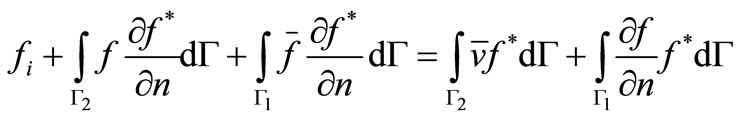
where by (-) are meant average values and Γ1, Γ2 are the boundaries in which the essential and the natural conditions are affected, respectively.
Beyond the above, integrating by parts the left hand side of Equation (3.1) follows:
 (3.2)
(3.2)
By integrating again the left hand side of Equation (3.2) one obtains:
 (3.3)
(3.3)
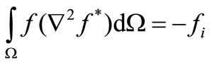
In order to find a solution satisfying the Laplace equation, then the governing equation is:
 (3.4)
(3.4)
where Δi is the Dirac delta function The solution of Equation (3.4) is called the fundamental solution and has the property such that:
 (3.5)
(3.5)
in which  is the value of the unknown function at the point “i” where a concentrated load is acting.
Thus, if Equation (3.4) is satisfied by the fundamental solution, then one has
 (3.6)
(3.6)
By using (3.6), then Equation (3.3) takes the form:
 (3.7)
(3.7)
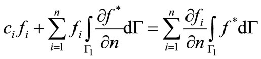
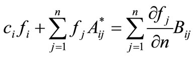
Furthermore, by taking the point “I” on the boundary, then the term fi in Equation (3.7) must be multiplied by 1/2 for a smooth boundary. On the other hand, if the boundary is not smooth at the point “I” then the number 1/2 must be replaced by a constant which can be determined from constant potential considerations.
Then Equation (3.7) takes the form:
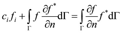 (3.8)
(3.8)
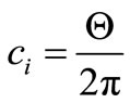
where Γ = Γ1 + Γ2 and has been assumed that f =`f on Γ1 and  on Γ2. Also, the constant ci can be determined by the relation:
 (3.9)
(3.9)
in which Θ denotes the internal angle of the corner in rad.
1) Constant Elements
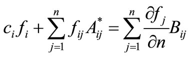
For the numerical evaluation of Equation (3.8) by using constant elements, then the above equation may be written as:
 (3.10)
Beyond the above, Equation (3.10) can be further written as:
 (3.11)
where 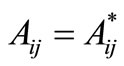 , when i ¹ j
 , when i = j (3.12)
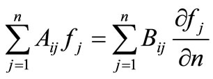
Hence, Equation (3.11) takes the form:
 (3.13)
or in matrix form may be written as:
 (3.14)
On the other hand, by reordering the above equation so that all the unknows are on the left hand side, then one has:
 (3.15)
where X is the vector of unknows f and v.
Thus, once the values of f and v on the whole boundary are known, then f can be calculated at any interior point:
 (3.16)
The integrals Bij and  can be calculated by using 4-point Gauss quadrature rule for the case
 . On the other hand, for the case i = j, because of the singularity needs a more accurate integration. Thus, for this case can be used higher-order integration or logarithmic formula.
2) Linear Elements
For the numerical evaluation of Equation (3.8) by using linear elements, then the above equation can be written as:
 (3.17)
In this case, in contrary to Equation (3.10), the variables fj and  cannot be taken out of the integral as they vary linearly within the element.
Thus, by using linear elements then Equation (3.17) can be further written as:
 (3.18)
By the same way, as for Equation (3.13), the above equation takes the form:
 (3.19)
and in matrix form:
 (3.20)
Finally, by using either constant or linear elements then the velocities v = ¶f/¶n are computed on the free surface of the spillway flow.
Also, the free surface elevations y, are further computed by the formula:
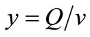 (3.21)
and thus the free-surface profile is fully determined.
4. Application to the Determination of the Free-Surface Profile of a Spillway
As an application of the previous outlined theory, the free-surface profile will be determined over a spillway of height h = 7.55 m, designed for a flow rate of 5.5 m3/sec/m of width. The same problem has been previously solved by A. H. D. Cheng, J. A. Liggett and P. L. F. Liu [14] by using the Boundary Integral Equation Method (B.I.E.M.) and by V. T. Chow [39] by using experimental results. Thus, a comparison will be made between the results of the Singular Integral Operators Method (S.I.O.M.), the B.I.E.M. and the experimental results. Furthermore, the flow rate Q can be changed as a function of time (Q = Q(t)) because of the unsteady flow, and for any different Q, then a different curve over the spillway occurs.
The problem has been solved by using both constant and linear elements. Hence, as it can be seen from Figure 2 the results of the linear elements by using the S.I.O.M., are in fair agreement with the coresponding results of the B.I.E.M. and the experimental curve. On the other hand, there is a small disagreement between the results of the constant elements of the S.I.O.M. and the corresponding methods. This is mainly explained by the fact that the constant elements are not well fitted in the zone of uncertainty of the flow over the spillway.
On the other hand, when the flow rate is changed per unit time, for the cases of a general uniform flow over the spillway, then different curves occur. Thus, there are no limits on the dimension of the flow problem that can be solved by the S.I.O.M. In these cases although the flows over the spillway are more complicated, the S.I.O.M. is well applied.
Although the Boundary Element Method has been used once in the past [14] for solving such a problem, the S.I.O.M. gives more accurate results with more complicated algorithms, which in any case are faster and more exact.
5. Conclusions
The Singular Integral Operators Method was applied to the determination of the free-surface profile of the unsteady flow over a spillway. This is very important problem of classical hydraulics and especially in open channel flow. Thus there are some basic parameters of the unsteady spillway flows, like the discharge, the free surfaces and speeds which are necessary for the design of the spillways. In the past such parameters were obtained through experiments, but the rapid development of the numerical techniques in hydraulics problems, made efficient the possibility of obtaining such parameters through computational methods.
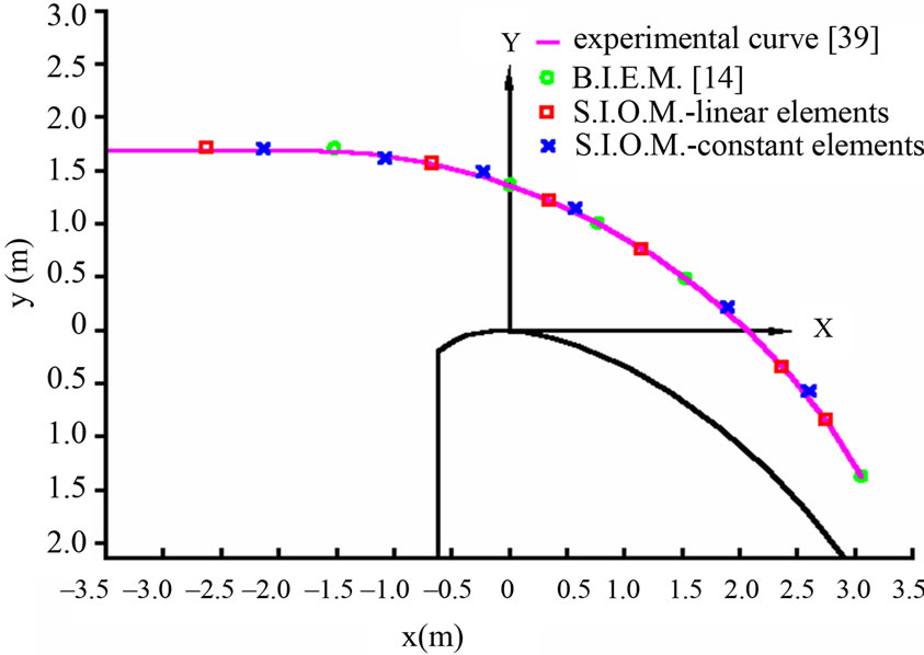
Figure 2. Surface Profile for a Spillway with Q = 5.5 m3/sec/m width.
The governing equation for solving potential flow problems is the equation of Laplace. So by using the Laplacean and choosing the proper boundary conditions, then the unsteady flows over a spillway are calculated by using a numerical techique based on the singular integral equations. For the numerical evaluation of the singular integral equations were used both constant and linear elements. An application was given to the determination of the free-surface profile of a special spillway and the results were compared with corresponding numerical results by the boundary elements and by using experiments.
Finally the proposed method by using the equation of Laplace for solving potential problems can be applied in several other hydraulics problems of open channel flows. Thus, in future special attention should be given to the research and application of the integral equation methods to the solution of several important problems of open channel hydraulics.
REFERENCES
- R. V. Southwell and G. Vaisey, “Relaxation Methods Applied to Engineering Problems: XIII, Fluid Motions Characterized by Free Streamlines,” Philosophical Transactions of the Royal Society of London. Series A, Mathematical and Physical Sciences, Vol. 240, No. 815, 1946, pp. 117-161.
- J. S. McNown, E.-Y. Hsu and C.-S. Yih, “Application of the Relaxation Technique in Fluid Mechanics,” Transactions of ASCE, Vol. 120, 1955, pp. 650-686.
- J. J. Cassidy, “Irrotational Flow over Spillways of Finite Height,” Journal of the Engineering Mechanics Division, Vol. 91, No. 6, 1965, pp. 155-173
- J. A. McCorquodale and C. Y. Li, “Finite Element Analysis of Sluice Gate Flow,” Engineering Journal, Vol. 54, No. , 1971, pp. 1-4.
- S. T. K. Chan, B. E. Larock and L. R. Hermann, “FreeSurface Ideal Fluid Flows by Finite Elements,” Journal of the Hydraulics Division, Vol. 99, No. 3, 1973, pp. 959- 974.
- M. Ikegawa and K. Washizu, “Finite Element Method Applied to Analysis of Flow over a Spillway Crest,” International Journal for Numerical Methods in Engineering, Vol. 6, No. 2, 1973, pp. 179-189. doi:10.1002/nme.1620060204
- L. T. Isaacs, “A Curved Triangular Finite Element for Potential Flow Problems,” International Journal for Numerical Methods in Engineering, Vol. 7, No. 3, 1973, pp. 337-344. doi:10.1002/nme.1620070310
- L. T. Isaacs, “Numerical Solutionfor Flow under Sluice Gates,” Journal of the Hydraulics Division, Vol. 103, No. 5, 1977, pp. 473-481.
- B. E. Larock, “Flow over Gated Spillway Crests,” Proceedings of 14th Midwestern Mechanics Conference, Vol. 8, University of Oklahoma Press, Norman, 1975, pp. 437- 451.
- H. J. Diersch, A. Schirmer and K. F. Busch, “Analysis of Flows with Initially Unknown Discharge,” Journal of the Hydraulics Division, Vol. 103, No. 3, 1977, pp. 213-232.
- E. Varoglu and W. D. L. Finn, “Variable Domain Finite element Analysis of Free Surface Gravity Flow,” Computes & Fluids, Vol. 6, No. 2, 1978, pp. 103-114. doi:10.1016/0045-7930(78)90011-7
- P. L. Betts, “A Variational Principle in Terms of Stream Function for Free-Surface Flows and Its Application to the Finite Element Method,” Computes & Fluids, Vol. 7, No. 2, 1979, pp. 145-153. doi:10.1016/0045-7930(79)90030-6
- J. A. Liggett, “Location of Free Surface in Porous Media,” Journal of the Hydraulics Division, Vol. 103, No. 4, 1977, pp. 353-365.
- A. H.-D. Cheng, J. A. Liggeand P. L.-F. Liu, “Boundary Calculations of Sluice and Spillway Flows,” Journal of the Hydraulics Division, Vol. 107, No. 4, 1981, pp. 1163- 1178.
- T. S. Strelkoff, “Solution of Highly Curvilinear Gravity Flows,” Journal of the Engineering Mechanics Division, 90, Vol. 90, No. 3, 1964, pp. 195-222.
- T. S. Strelkoff and M. S. Moayeri, “Patern of potential Flow in a Free Surface Overfall,” Journal of the Hydraulics Division, Vol. 96, No. 4, 1970, pp. 879-901.
- Y. Guo, X. Wen, C. Wu and D. Fang, “Numerical Modelling of Spillway Flow with Free Drop and Initially Unknown Discharge,” Journal of Hydraulic Research, Vol. 36, No. 5, 1998, pp. 785-801. doi:10.1080/00221689809498603
- E. G. Ladopoulos, “Finite—Part Singular Integro—Differential Equations Arising in Two-Dimensional Aerodynamics,” Archives of Mechanics, Vol. 41, 1989, pp. 925- 936.
- E. G. Ladopoulos, “Non-Linear Singular Integral Representation for Unsteady Inviscid Flowfields of 2-D Airfoils,” Mechanics Research Communications, Vol. 22, No. 1, 1995, pp. 25-34. doi:10.1016/0093-6413(94)00036-D
- E. G. Ladopoulos, “Non-Linear Singular Integral Computational Analysis for Unsteady Flow Problems,” Renewable Energy, Vol. 6, No. 8, 1995, pp. 901-906. doi:10.1016/0960-1481(95)00099-1
- E. G. Ladopoulos, “Non-Linear Singular Integral Representation Analysis for Inviscid Flowfields of Unsteady Airfoils,” International Journal of Non-Linear Mechanics, Vol. 32, No. 4, 1997, pp. 377-384. doi:10.1023/A:1004246318082
- E. G. Ladopoulos, “Non-Linear Multidimensional Singular Integral Equations in 2-Dimensional Fluid Mechanics Analysis,” International Journal of Non-Linear Mechanics, Vol. 35, No. 4, 2000, pp. 701-708.
- E. G. Ladopoulos, “Non-Linear Unsteady Flow Problems by Multidimensional Singular Integral Representation Analysis,” International Journal of Mathematics and Mathematical Sciences, Vol. 2003, No. 50, 2003, pp. 3203- 3216.
- E. G. Ladopoulos, “Non-Linear Two-Dimensional Aerodynamics by Multidimensional Singular Integral Computational Analysis,” Forshung im Ingenieurwesen, Vol. 68, No. 2, 2003, pp. 105-110. doi:10.1007/s10010-003-0114-7
- E. G. Ladopoulos, “Singular Integral Equations, Linear and Non-Linear Theory and its Applications in Science and Engineering,” Springer, Berlin, 2000.
- E. G. Ladopoulos, “Singular Integral Equations in Potential Flows of Open-Channel Transitions,” Computes & Fluids, Vol. 39, No. 9, 2010, pp. 1451-1455. doi:10.1016/j.compfluid.2010.04.013
- E. G. Ladopoulos and V. A. Zisis, “Existence and Uniqueness for Non-Linear Singular Integral Equations Used in Fluid Mechanics,” Applications of Mathematics, Vol. 42, No. 5, 1997, pp. 345-367. doi:10.1023/A:1023058024885
- E. G. Ladopoulos and V. A. Zisis, “Non-Linear Finite-Part Singular Integral Equations Arising in Two-Dimensional Fluid Mechanics,” Nonlinear Analysis: Theory, Methods & Applications, 42, Vol. 42, No. 1, 2000, pp. 277-290.
- E. G. Ladopoulos, “On the Numerical Evaluation of the Singular Integral Equations Used in Twoand Three-Dimensional Plasticity Problems,” Mechanics Research Communications, Vol. 14, No. 4, 1987, pp. 263-274. doi:10.1016/0093-6413(87)90039-5
- E. G. Ladopoulos, “Singular Integral Representation of Three-Dimensional Plasticity Fracture Problem,” Theoretical and Applied Fracture Mechanics, Vol. 8, No. 3, 1987, pp. 205-211. doi:10.1016/0167-8442(87)90047-4
- E. G. Ladopoulos, “On the Numerical Solution of the Multidimensional Singular Integrals and Integral Equations Used in the Theory of Linear Viscoelasticity,” International Journal of Mathematics and Mathematical Sciences, Vol. 11, No. 3, 1988, pp. 561-574. doi:10.1155/S0161171288000675
- E. G. Ladopoulos, “Singular Integral Operators Method for Two-Dimensional Plasticity Problems,” Computer & Structures, Vol. 33, No. 3, 1989, pp. 859-865. doi:10.1016/0045-7949(89)90260-5
- E. G. Ladopoulos, “Cubature Formulas for Singular Integral Approximations Used in Three-Dimensional Elasticity,” Revue Roumaine des Sciences Techniques. Série de Mécanique Appliquée, Vol. 34, No. 4, 1989, pp. 377-389.
- E. G. Ladopoulos, “Singular Integral Operators Method for Three-Dimensional Elasto-Plastic Stress Analysis,” Computer & Structures, Vol. 38, No. 1, 1991, pp. 1-8. doi:10.1016/0045-7949(91)90117-5
- E. G. Ladopoulos, “Singular Integral Operators Method for Two-Dimensional Elasto-Plastic Stress Analysis,” Forshung im Ingenieurwesen, Vol. 57, No. 5, 1991, pp. 152- 158. doi:10.1007/BF02561415
- E. G. Ladopoulos, “Singular Integral Operators Method for Anisotropic Elastic Stress Analysis,” Computer & Structures, Vol. 48, No. 6, 1993, pp. 965-973. doi:10.1016/0045-7949(93)90431-C
- E. G. Ladopoulos, “3-D Elastostatics by Coupling Method of Singular Integral Equations with Finite Elements,” Engineering Analysis with Boundary Elements, Vol. 26, No. 2, 2002, pp. 591-596 doi:10.1016/S0955-7997(02)00021-8
- E. G. Ladopoulos, “Coupling of Singular Integral Equation Methods and Finite Elements in 2-D Elasticity,” Forshung im Ingenieurwesen, Vol. 69, No. 1, 2004, pp. 11-16. doi:10.1007/s10010-004-0131-1
- V. T. Chow, “Open Channel Hydraulics,” McGraw-Hill, New York, 1959.
Nomenclature
f stream function;
Q flow rate per unit width;
v velocity;
n unit normal from the free surface;
g acceleration of gravity;
y free surface elevation;
H design load;
f* weighting function;
Γ1 boundary in which the essential conditions are affected;
Γ2 boundary in which the natural conditions are affected;
Δi dirac delta function;
Θ internal angle of the corner in rad.