Engineering
Vol. 3 No. 6 (2011) , Article ID: 5696 , 4 pages DOI:10.4236/eng.2011.36066
Uniaxial Modelling of Behavior of the Concrete in Fast Dynamics: Approach to Seismic Behavior
1University of Bechar, Bechar, Algeria
2University of Oran, Oran, Algeria
E-mail: numelab@yahoo.fr
Received December 2, 2010; revised May 20, 2011; accepted June 3, 2011
Keywords: Concrete, Viscous-damage, strain rate
ABSTRACT
The advantages of the computer enable us to simulate of complex structures subjected to dynamic loading. To come up to the necessity to know the real behavior of such material, we exploit these advantages basing on experimental data available in the literature. Since the response of the material depends on stress velocity, so it is essential to provide a computational code with dynamic behavior. To perform such simulations, we have elabo-rated a behavior law governed by loading velocity effect on concrete and their attitudes cyclic non elastic, for an approach of seismic behavior. This paper shows the processes we have followed to formulate this viscous damage law whose aim is behavior prediction for concrete under dynamic stresses. Then, the model is validated with experimental results and simulations of some available tests on Hopkinson’s bar.
1. Introduction
Under rapid and dynamic impacts, concrete shows a mechanical behavior, particularly sensitive to rate loading [1-5]. These conditions leave the models simplified by static computations, even balanced by safety coefficients, unrealistic. Hence dynamic behavior analysis of concrete structures requires the use of models and laws that take into account a certain number of essential phenome-na relative to such situations.
Among the available approaches in literature, we have adopted a phenomenological thermodynamic approach to describe the damaged non linear hysteretic behavior of concrete, an approach used by Laborderie [6].
This approach has been developed to simulate the behavior of concrete structures subjected to monotonous or cyclic alternated loading quasi-static mode [6,7]; that is to say at a strain rate lower than 1 S-1. Within the frame of dynamic behavior simulation of concrete subjected essentially to seismic stresses, then under other types of impacts (blasts, percussion…), we will adapt this model to these types of stimulations. But this cannot be possible unless we introduce viscous effect induced by the high loading rates on materials.
2. Coupling of the Model to Viscosity
With reference to Dubé works [8], who had adopted for such pairing Perzyna’s viscosity model [9], many researchers expressed concrete viscosity through parameters given in terms of rate strain variations [10-14]. The introduction of velocity effect in our damage model, was done through a non dimensional parameter whose variation is linked first to dynamic increase factor (non dimensional) which is itself expressed in terms of strain rate.
This viscosity parameter noted “h”, will be paired with adjusting parameter noted “a”, hence the threshold function becomes:
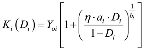 (1)
(1)
where:
Yoi: initial sill of damage.
ai, bi: positive real parameters to be determined by adjusting.
In case of dynamic behavior, damage variable is calculated by means of the following equation:
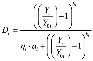 (2)
(2)
3. Establishing of the Uniaxial Model for the Concrete
Using isotropy hypothesis to describe concrete behavior in monoaxial model, will simplify the equation form, from a tonsorial writing to a scalar writing, hence the deformation will be written as follows:
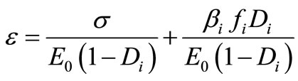 (3)
(3)
The stress is given by the following formula:
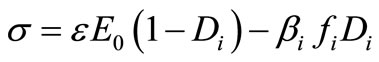 (4)
(4)
Hence the development law that we adopt for damage parameter “D”, is the one given by (2).
The Rate of voluminal refund of energy is expressed by the following equation:
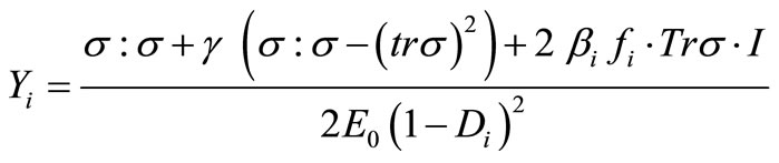 (5)
(5)
This rate takes the following uniaxial form:
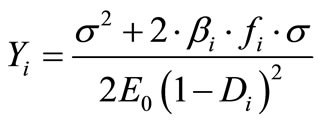 (6)
(6)
We express Yi in terms of deformations, by substituting (4) in (6):
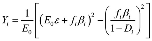 (7)
(7)
4. Determination of the Parameters
In this computational model [6,7,15], it is necessary to determine the following parameters:
E0; fi; bi: respectively, the modulus of elasticity in its origin; compressive strength or tensile strength in static behavior and the parameter of non-elasticity determined in static; all given starting from the experimental curve.
ai, bi: non dimensional parameters characterizing the damage variable determined by adjustment on the curve of experimental behavior in static.
Y0i: the initial threshold of damage:
In compression, it has been considered more convenient to take into account that the damage begins once exceeding concrete elastic stress in quasi static state [7], that is to say
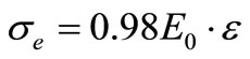 (8)
(8)
Taking se from par (8) and putting Dc = 0 in the equation (6), we have:
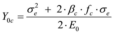 (9)
(9)
The initial threshold of damage in tension is considered once it attains 90% of the tensile strength stress of concrete ft [14]. By substituting se = 0.90 ft and Dt = 0 in the equation (6), we get:
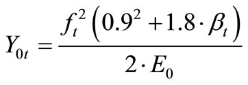 (10)
(10)
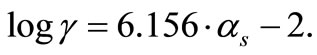
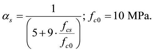
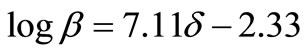
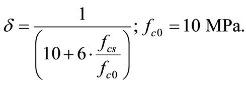
ηi: non dimensional material parameter of viscosity, calculated in terms of dynamic increase factor (DIF) in compression or tension.
5. The Parameter of Viscous Work Hardening ηii
The parameter hi influences the viscous response of concrete behavior in compression or tension. Governed by the deformation velocity variation, it gives the form of the curve after work hardening. The expression of viscous work hardening value directly in terms of strain rate  remains possible, but complicated. This is why, we express viscosity parameters in terms of dynamic increase factor (DIF) noted “”, which is it self estimated from strain rate and resistance characteristic of the concrete in static in CEB-FIP formula [16]. Basing on the experimental curves of Gary [17], Bishoff [2] and those of Cotsovos [18] in compression and on experimental works of dynamic tension of Brara [4] and Toutlemonde [19,20], also by the use of analytical relations of Ngo [21] to verify the fitting of deformation increase in terms of tensile stress increase; we have concluded that hi evolvement can be described by an equation of the form:
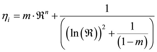 (11)
(11)
where, m and n are determined from two behavior charts obtained in dynamics under different strain rate bt resolving a non linear system of two equations with two unknowns.
6. Dynamic Increase Factor (DIF) R
fi: Dynamic resistance obtained to  (i = compression or tension).
fis: static resistance obtained to  (i = compression or tension).
Â: Dynamic increase factor (DIF).
6.1. In Compression
We use CEB-FIP formula [16] to assess dynamic increase factor value in compression:
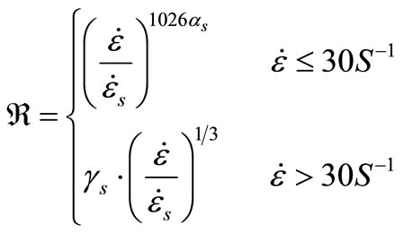 (12)
(12)
 : Strain rate, at a range of 30 × 10−6 to 300 S−1.
 : Static strain rate, at a range of 30 × 10−6.
6.2. In Tension
The assessment of dynamic increase factor values in tension is performed through CEB-FIP formula [16]:
 (13)
(13)
 : Strain rate, at a range 3 × 10⁻⁶ to 300 S−1.
 : Static strain rate, at a range 3 × 10⁻⁶.
7. Evolution of the Deformations and Rupture Criterion
In damage mechanics, the parameter “D” is usually the privileged indicator of the rupture once it reaches the value of “1”. Yet, as the model is for uniaxial behavior of a fragile material such as concrete, we can adopt a rupture criterion by deformation. The deformation sill of dynamic failure “ ”, is assessed in terms of failure sill by static deformation “
 ” combined with a strain rate
 . This was done under several types of formulations, either directly in terms of strain rate as one suggested by J. Mazars [22], or in terms of dynamic increase factor as shown in Ngo and Mendis [21]. Concerning our model, we suggest the description of the amplifications of deformations indirectly in terms of strain rate using the following relation:
 (14)
(14)
With: , if
, if .
.
The parameters m' and n' are determined by adjusting from two behavior curves (two charts are sufficient) obtained under dynamic tests.
8. Simulation of the BRARA’s Tensile Tests by Chipping
In 1997; the tensile tests by chipping were realized in the university of Metz on samples concrete MB50. High impact speeds (up to  = 130 S−1) that permitted to have the chipping of the concrete specimens, were reached by Hopkinson’s Bar [4,23]. Hopkinson’s Bar assembling of this test is based on the ejection of a projectile that hits an impact bar at a high speed, producing wave spreading through the impact bar and the sample, which generates a pulling on the free side of the sample.
The samples are designed in cylindrical form, which is 40 mm in diameter and has length of 120 mm. They are impacted by a metallic cylinder (entry bar) that has the same section with one meter in length (Figure 1).
These samples in MB50, concrete have the following characteristics (Table 1):
Under two different impact velocities, the experiments we have simulated are divided into two notations: BE16 test, the slowest with a strain rate of 35.9 (S−1); and BE12 test whose strain rate is about two times BE16’s.
8.1. BE16, BE12 Tests
The BE16 is the slowest test, its impact velocity equals 7.
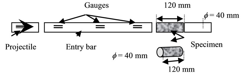
Figure 1. Experimental assembling of tensile tests on Hopkinson’s bar.
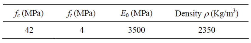
Table 1. Mechanical characteristics of the concrete used in Brara’s tests.
m·s−1, generating a strain rate that equals  = 35.9 S−1. Under these conditions the specimen has shown a single failure during time period of 7.2 10−5 S at a distance of 65.8 mm from the free edge. Rupture dynamic stress is estimated at std = 19.2 MPa.
The BE12 test has an impact velocity that equals 15 m·s−1, generating a strain rate equals  = 70.4 S−1. After a time period exceeding significantly 5 × 10⁻⁵ S, two fissures appear at the distances of 41 mm and 69 mm from the free edge. Rupture dynamic stress is esteemed at std = 33.5 MPa around 69 mm.
8.2. Model Adjusting
The determination of the different parameters essential to the calculations, and achieved by adjusting on the static curve, has given the following values at = 3.55 and bt = 1.00. The static behavior chart made by our model has got the form shown in figure (Figure 2).
After adjusting to dynamic behavior data, viscous parameters took the following values mt = 0.0283 and nt = 5.0617. Model response to different strain rate is shown on the figure (Figure 3).
8.3. Numerical Simulation of the Tests
Finite elements grid we used, has a fiber of 1 mm alongside the sample (120 fibers). Such discretization enables us to follow the development of mechanical characteristics with time in their locations with an accuracy of about 1 mm. Concerning the boundary conditions of the specimen, the blocking up happens on the impacted side; however the free side bears the applied experimental velocity.
8.3.1. BE16 Test Simulation
This simulation provided us with a very rapid movement
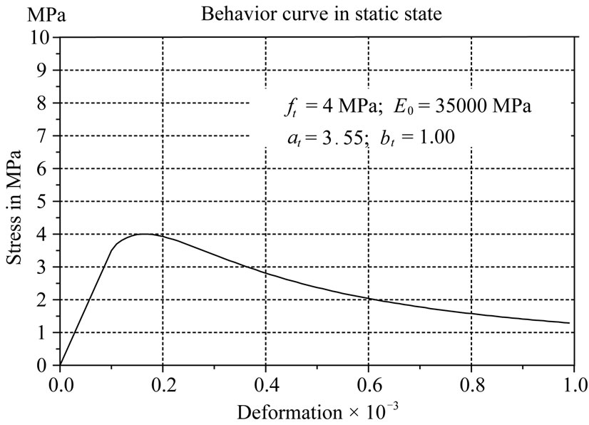
Figure 2. Static behavior curve of be samples made by our model with values of at = 3.55 and bt = 1.00.
of the damage. The parameter “D” evolves to be important once impact time reaches the value 4 × 10⁻⁵ S, but the ultimate value of “1” is reached only at 7.2 × 10⁻⁵ S, at the 61st fiber at a distance of 59 mm from the free edge (Figure 5). This value indicates the position of the micro fissure that causes the rupture, at a gap of 6 to 7 mm of experimental failure position (65.8 mm from the free edge). The time of rupture in the simulation appearance is identical to the experimental one (7.2 × 10⁻⁵ S). At first, stress diffusion through the cylinder happens as if it was under static loading, but after a certain period of time, stress development evolves with time in each fiber separately from the others, the simulated rupture stress stdr equals 19.09 MPa (Figure 6), knowing that the experimental value is stdr = 19.2 MPa.
Finally, we turn attentions on input force in the simulation. This force obtains the maximum value of 4.3 × 10⁴ N, in a time period of t = 3.25 × 10⁻⁵ S, allows the comparison between experimental and simulated values (Table 2).
8.3.2. BE12 Test Simulation
Under an impact velocity V0 = 15 m·s−1 and given strain rate that equals  = 70.4 S−1, BE12 test simulation has shown that “D” ultimate value of “1” is reached successively and almost simultaneous in two locations, indicat-
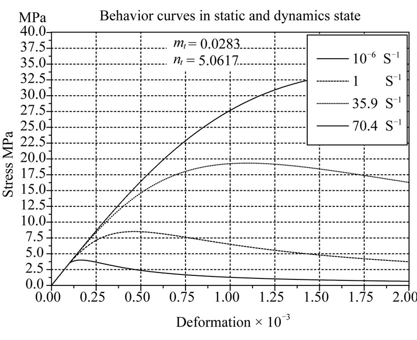
Figure 3. Model reponses under different strain rate obtained with the parameters mt = 0.0283 and nt = 5.0617.
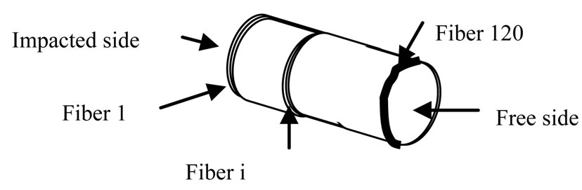
Figure 4. Sample discretization in 1 mm fibers.
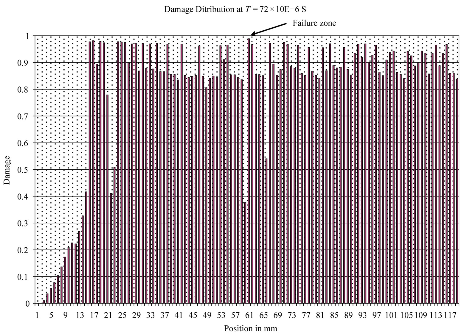
Figure 5. Simulated damage distribution at T = 7.2 × 10⁻⁵ S.
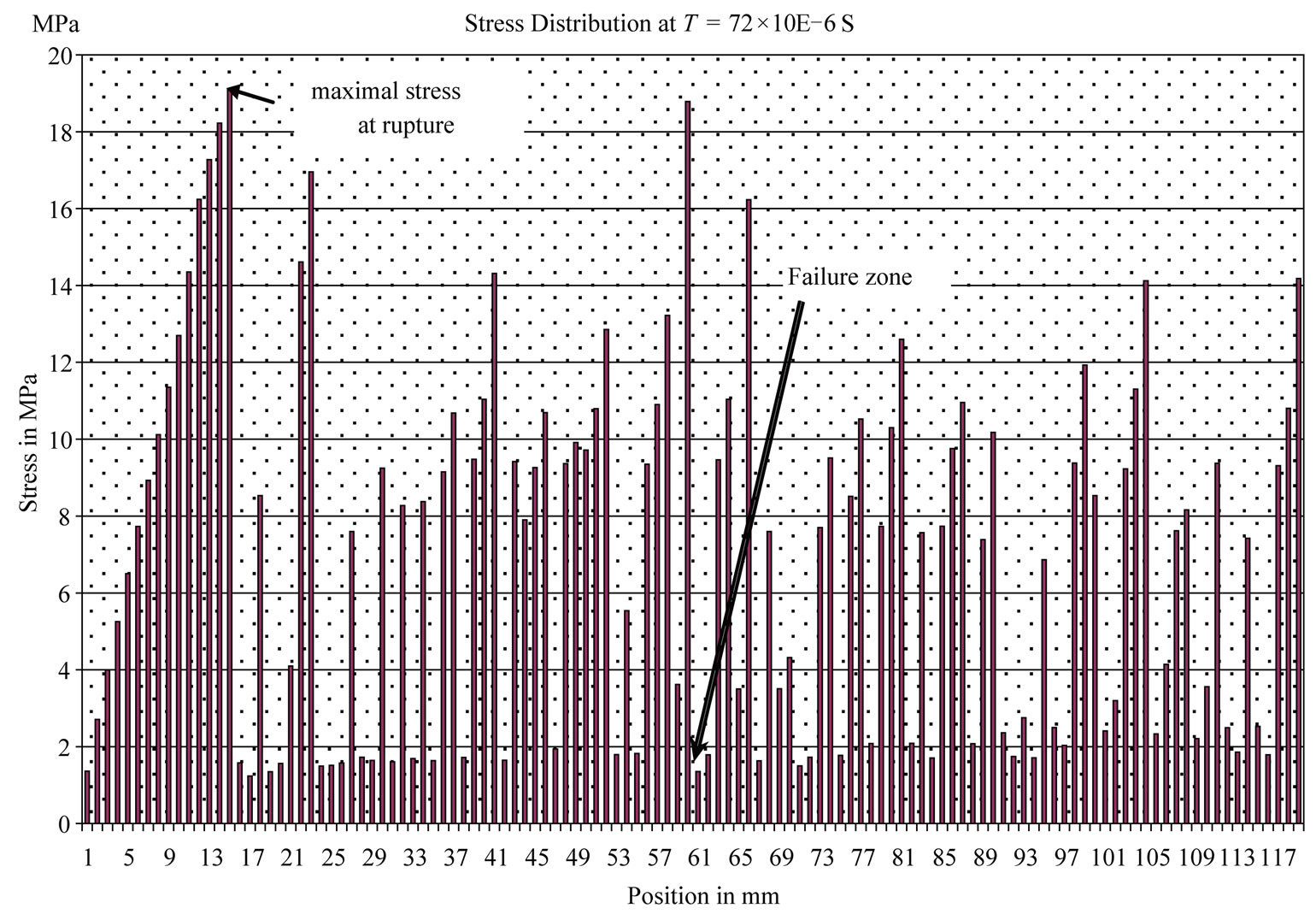
Figure 6. Simulated stresses distribution at rupture at T = 7.2 × 10⁻⁵ S.
ing the starting of two successive failures at the time t = 4.94 × 10⁻⁵ S. The first one appeared in the 51st fibber, making a distance of 69 mm from the free edge. The second appeared in the 79th fiber, at a distance of 41 mm from free edge (Figure 7). These values show a good conformity between simulated and experimental results. The maximum value of the simulated rupture stress stdr equals 33.52 MPa (Figure 8). It is to be noted that this stress is obtained since the starting of the first failure (51st fiber ) as our computational code stops automatically once the damage is full filled in a given fiber (D = 1). The model gives an input force value of 7.5 × 10⁴ N in a time period that equals t = 1.63 × 10⁻⁵ S. The table (Table 3) shows the results obtained by model simulation and experimental one.
9. Conclusions
The development of the model has been achieved by introducing viscosity in damage evolvement, a fact which allowed the regulation of dynamic problems and the reproduction of velocity effects noticed in the experiments. In the basic model we have used, we introduced viscous parameters by reproducing concrete behavior with dynamic stimulation, according to the available experimental results in literature.
In practice, our model contains four parameters to identify by adjusting on experimental data, which has
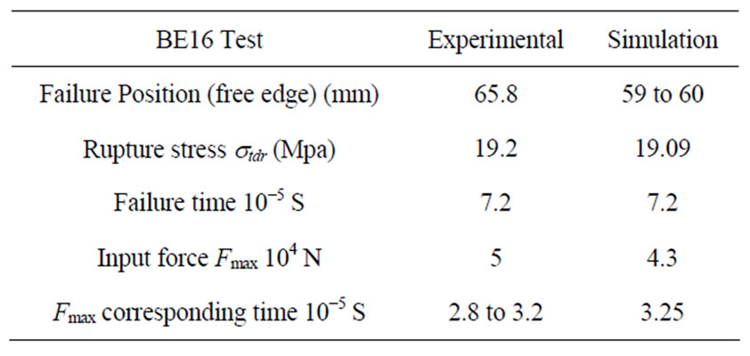
Table 2. A comparison between BE16 test experimental and simulation values.
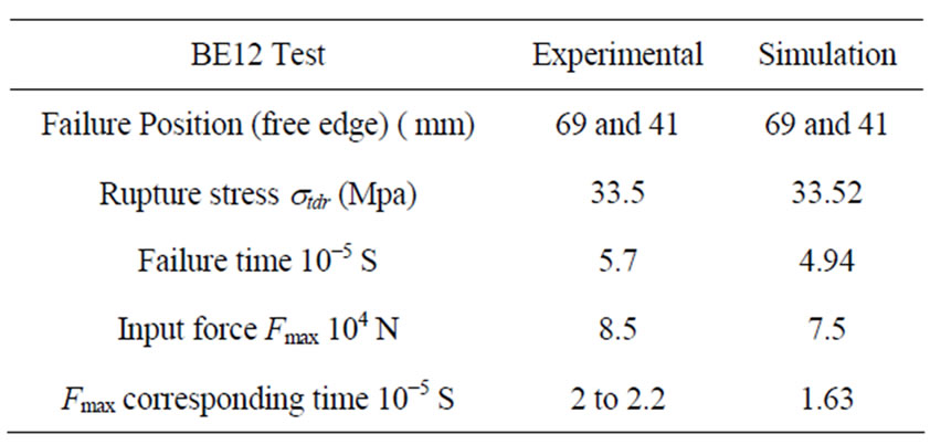
Table 3. A comparison between BE12 test experimental results and their simulations.
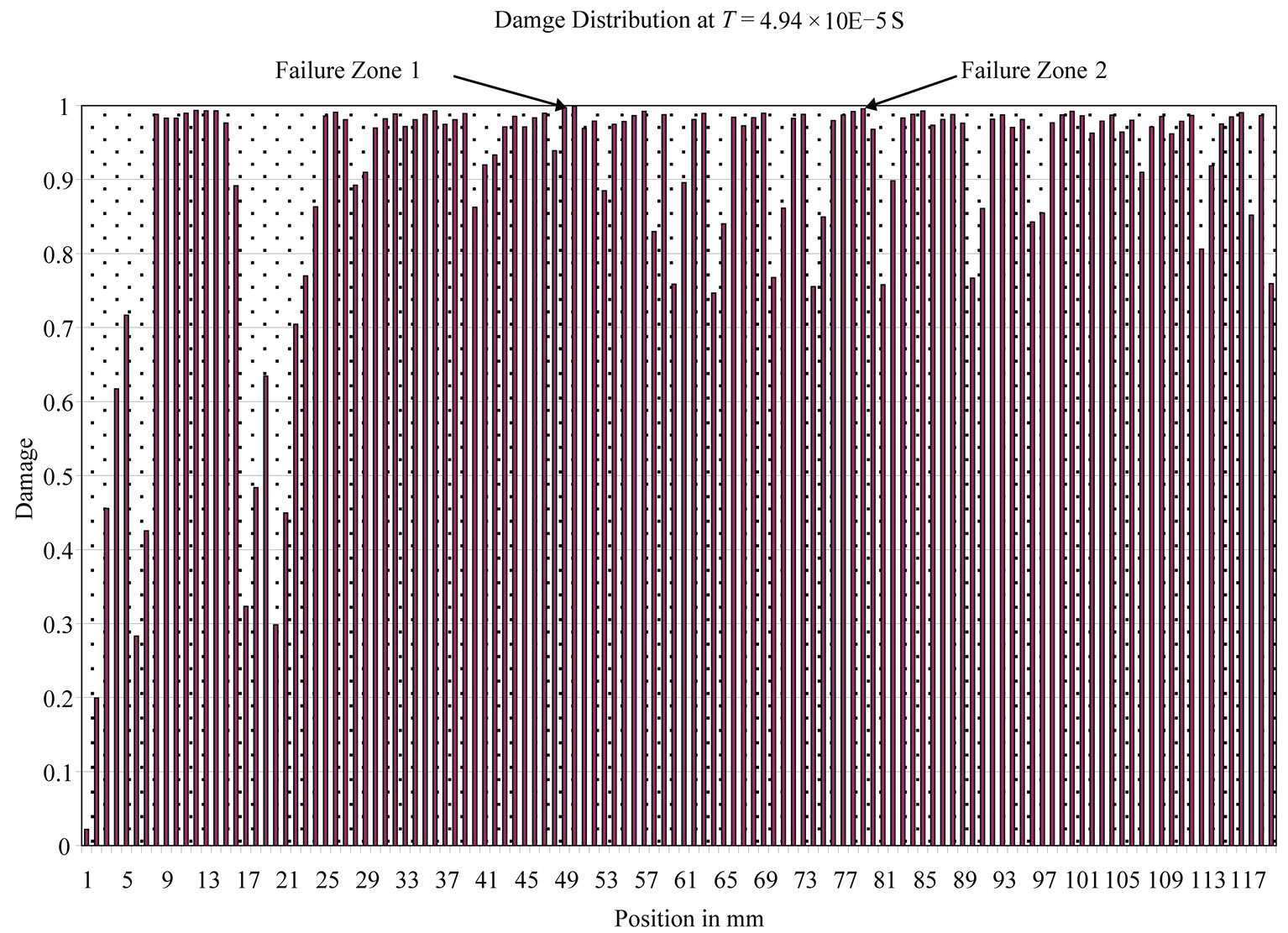
Figure 7. Simulated damage distribution at T = 4.94 × 10⁻⁵ S of BE12 sample.
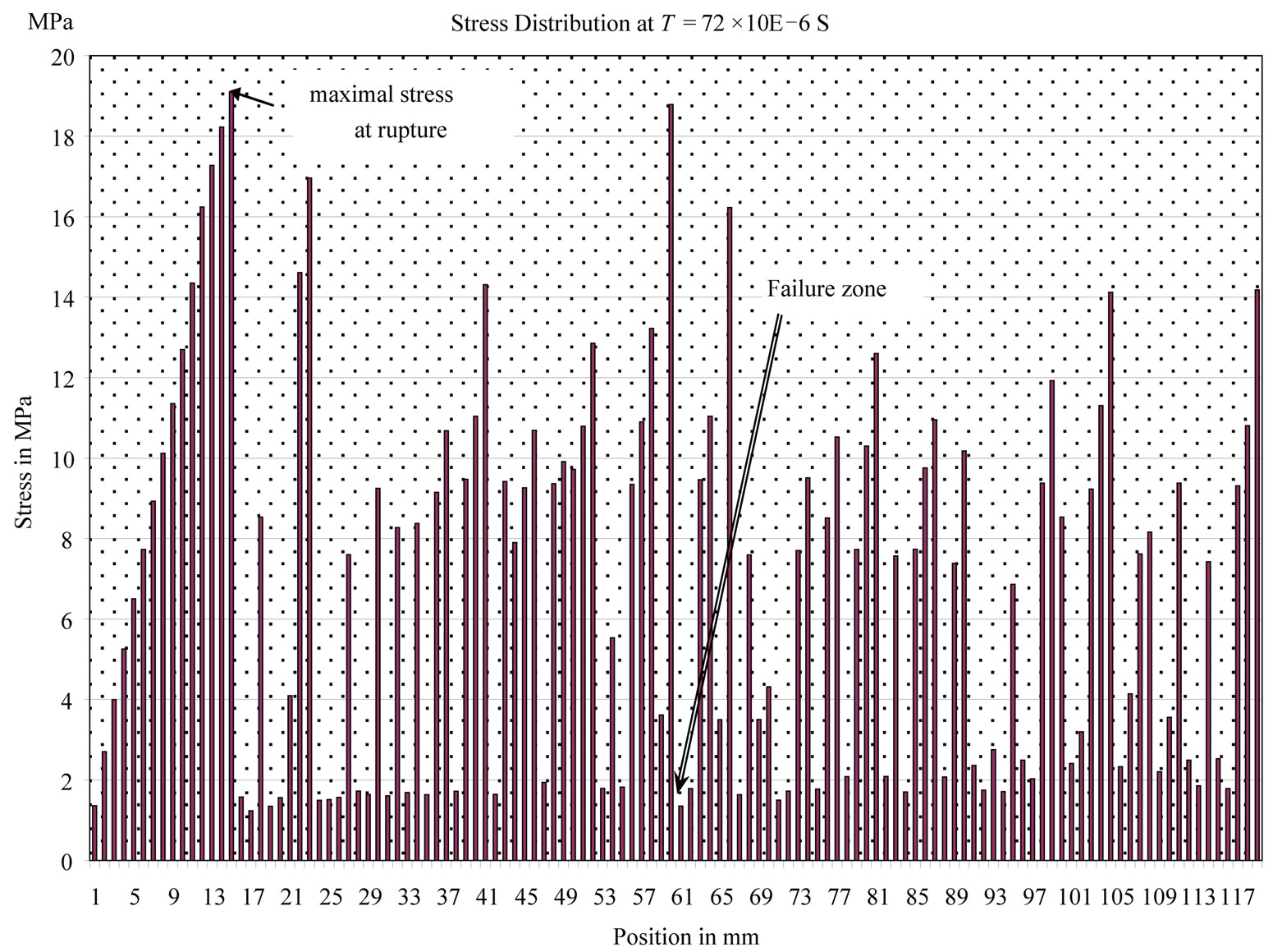
Figure 8. Simulated stresses distribution in rupture at T = 4.94 × 10⁻⁵ S of BE12 sample.
been the case for the majority of the models suggested in that way, except the fact that our model has the advantage of estimating dynamic increase factor trough a first law elaborated by means of experiments namely (CEBFIP) formula. Then, a second adjustment has been performed for each concrete, in terms of its own response to dynamic loading, because viscosity problem is not totally surrounded by (CEB-FIP) formula since many concretes don’t follow this law faithfully in their dynamic increase factor.
Finally, the developed model agreement with different experiments has proved its performance in the description of concrete dynamic behavior. Being implemented in a calculation code of structures in finite elements, it guarantees both the follow up of structures response in real time and after the disappearance of actions, that is to say the assessment of residual deformations at the time of failure.
The model is practically useful for the simulation of alternated cyclic behavior in rapid dynamics, which will allow the reproduction of the attitudes of structures subjected to seismic stresses.
In a future prospect, we hope expanding the model to take into account deviation effects in an anisotropic continuous medium like the concrete.
• This model can be adapted to other materials whose behaviors are close to concrete behavior (fragile behavior), i.e.: rocks, ceramics, etc.
• Pairing the model with heat transfer effects that take place in certain impacts especially blasts.
• Taking into account some mechanical phenomena occurring when every concrete structure is under action like for example plastic deformation and fatigue.
10. REFERENCES
- H. Reinhard, “Influence of Stress-Rate and Strain-Rate on Mechanical Properties of Concrete,” CEB GTC, 14 Impact and Impulsive Loading of Concrete Structures, 1985.
- P. Bishoff and S. Perry, “Compressive Behaviour of Concrete at High Strain Rates,” Materials and Structures, Vol. 24, No. 6, 1991, pp. 425-450. doi:10.1007/BF02472016
- C. Denoual, “Probabilistic Approach of the Impact Behavior of Silicon Carbide: Application to Shielding Means,” Thesis, Ecole Normale Superieure, Cachan, France, 1998.
- A. Brara, “Experimental Study of the Dynamic Tension of Concrete by Spalling Thesis,” University of Metz, Metz, 1999.
- F. Camborde and C. Mariotti, “Study of Dynamic Behavior of Brittle Materials by Discrete Elements,” 14 Congress of Mechanics Toulouse, France, 1999.
- C. Laborderie, “Phenomena in Unilateral Material Damaged Modeling and Application to the Analysis of Concrete Structures,” Thesis, University of Paris VI, France, 1991.
- M. Benmansour, “Modeling the Behavior of Cyclic Alternating BA under Various Static Tests of Poles,” Thesis, ENPC Ecole, Paris, France, 1997.
- J. F. Dubé, “Simplified Model Behavior and Visco-Damaged Concrete Structures,” Thesis, Ecole Normale superieure, Cachan, France, 1994.
- P. Perzyna, “Fundamental Problems in Viscoplasticity,” Advances in Applied Mechanics, Vol. 9, 1966, pp. 935- 950.
- J. C. Simo, T. Hughes, “Computational Inelasticity-Interdisciplinary Applied Mathematics,” Springer-Verlag, New York, 1998.
- F. Gatuingt, “Predicting Fracture of Concrete Structures Sought in Fast Dynamic,” Thesis, Ecole Normale superieure, Cachan, France, 1999.
- A. Winnicki, C. J. Pearce and N. Bicanic, “Viscoplastic Hoffman Consistency Model for Concrete,” Computers & Structures, Vol. 79, No. 1, 2001, pp. 7-19. doi:10.1016/S0045-7949(00)00110-3
- C. Laborderie, “Strategies and Models for Calculations Concrete Structures,” Thesis, University of Pau, Paris, France, 2003.
- F. Barpi, “Impact Behavior of Concrete: Computational Approach,” Engineering Fracture Mechanics, Vol. 71, No. 15, 2004, pp. 2197-2213. doi:10.1016/j.engfracmech.2003.11.007
- A. Baraka, “Contribution to the Modeling of Cyclic Behavior of Concrete Alternate with the Damage Mechanics,” Thesis, University of Sciences and of Technology, Oran, Algeria, 2002.
- CEB-FIP, “CEB-FIP Model Code 1990,” Trowbridge, Wiltshire, UK, 1993.
- G. Gary, “Tests at High Speed on Concrete,” Specific problems GRECO Publisher, Paris, 1990.
- D. Cotsovos, “Numerical Investigation of Structural Concrete under Dynamic (Earthquake and Impact) Loading,” Thesis, University of London, London, 2004.
- F. Toutlemonde, “Impact Resistance of Concrete Structures, the Behavior of the Material Costing,” Thesis, ENPC Ecole, Paris, France, 1995.
- F. Toutlemonde, J. Sercombe, J-M. Torrenti and R. Adeline, “Development of a Container for the Storage of Nuclear Waste: Impact Resistance,” Edition Hermès, Revue française de génie civil, Vol. 3, 1999, pp. 729-756.
- T. D. Ngo, P.A. Mendis, D. Teo and G. Kusuma, “Behavior of High-Strength Concrete Columns Subjected to Blast Loading,” University of Melbourne, Melbourne, 2002.
- J. Mazars, “Recent Developments in Search for Models ‘Comprehensive’ Models ‘Simplified’ for Reinforced Concrete Structures under Severe Stress,” Numerical Modeling and Engineering of Construction, Paris, 2005.
- A. Brara and J. R Klepaczko “New Experimental Study of Rupture of Concrete Spalling,” Communication Congress GEO, France, 1997.