Intelligent Control and Automation
Vol.08 No.04(2017), Article ID:81090,23 pages
10.4236/ica.2017.84014
Hamiltonian Servo: Control and Estimation of a Large Team of Autonomous Robotic Vehicles
Vladimir Ivancevic1, Peyam Pourbeik2
1Joint and Operations Analysis Division, Defence Science & Technology Group, Canberra, Australia
2CEWD, Assured Communications, Survivable Networks, Defence Science & Technology Group, Adelaide, Australia

Copyright © 2017 by authors and Scientific Research Publishing Inc.
This work is licensed under the Creative Commons Attribution International License (CC BY 4.0).
http://creativecommons.org/licenses/by/4.0/


Received: November 7, 2017; Accepted: November 27, 2017; Published: November 30, 2017
ABSTRACT
This paper proposes a novel Hamiltonian servo system, a combined modeling framework for control and estimation of a large team/fleet of autonomous robotic vehicles. The Hamiltonian servo framework represents high-dimensional, nonlinear and non-Gaussian generalization of the classical Kalman servo system. After defining the Kalman servo as a motivation, we define the affine Hamiltonian neural network for adaptive nonlinear control of a team of UGVs in continuous time. We then define a high-dimensional Bayesian particle filter for estimation of a team of UGVs in discrete time. Finally, we formulate a hybrid Hamiltonian servo system by combining the continuous-time control and the discrete-time estimation into a coherent framework that works like a predictor-corrector system.
Keywords:
Team of UGVs, Kalman Servo, Hamiltonian Control, Bayesian Estimation

1. Introduction
Today’s military forces face an increasingly complex operating environment, whether dealing with humanitarian operations or in the theater of war. In many situations one has to deal with a wide variety of issues from logistics to lack of communications infrastructure [1] . In many situations one may be even denied satellite access and hence unable to utilize services such as GPS for Geo-location and the ability reconnect back to HQ [2] .
Given the increasing success of artificial intelligence (AI) techniques in recent times and the advancements made in unmanned vehicle (UV) design, autonomous systems in particular teams or swarms of autonomous vehicles have become a potential attractive solution to solving the complexity issues facing the military today. Teams or swarms of intelligent autonomous vehicles would also introduce a level of survivability to the systems which would increase its utility in such complex and hostile environments [3] .
A problem which arises in utilizing large teams or swarms of autonomous vehicles is one of control. Recently, the US Defence Advanced Research Projects Agency (DARPA) has sought to address some of the control issues associated with large swarm through its Offensive Swarm-Enabled Tactics (OFFSET) [4] . Therefore, there is a clear need for both local and global control of large teams or swarms of UV. This would allow for autonomous or semi-autonomous operation of large teams of UV which would be easily manageable.
This paper proposes a Hamiltonian servo system which is a combined modeling framework for the control and estimation of such autonomous teams of UV’s. This paper will demonstrate the ability of this framework to handle the high-dimensional, nonlinear and non-Gaussian nature of the problem at hand. The authors will also show this to be a generalization of the classic Kalman Servo System. Finally results of a number of simulations will be presented to demonstrate the validity of the framework through the authors implementation using Mathematica & C++ code (which is provided in the Appendix).
Slightly more specifically, we recall here that traditional robotics from the 1970s-80s were mainly focused on building humanoid robots, manipulators and leg locomotion robots. Its modeling framework was linear dynamics and linear control, that is, linearized mechanics of multi-body systems (derived using Newton-Euler, Lagrangian, Gibs-Appel or kinetostatics equations of motion) and controlled by Kalman’s linear quadratic controllers (for a comprehensive review, see [5] - [11] ). The pinnacle of this approach to robotics in the last decade has been the famous Honda robot ASIMO (see [12] ), with a related Hamiltonian biomechanical simulator [13] .
In contrast, contemporary robotics research has mainly been focused on field robotics, based on estimation rather than control, resulting in a variety of self-localization and mapping (SLAM) algorithms (see [14] [15] [16] [17] [18] and the OpenSLAM web-site [19] ).
Instead of following one of these two sides of robotics, in the present paper we will try to combine them. From a robotics point-of-view, control and estimation are two complementary sides, or necessary components, of efficient manipulation of autonomous robotic vehicles. In this paper we attempt to develop a computational framework (designed in Wolfram MathematicaÒ and implemented in C++) that unifies both of these components. From a mathematical point-of-view, in this paper we attempt to provide nonlinear, non-Gaussian and high-dimensional generalization of the classical Kalman servo system, outlined in the next section.
2. Motivation: Kalman Servo
In 1960s, Rudolf Kalman developed concept of a controller-estimator servo

Figure 1. Kalman’s fundamental controller-estimator servo system, including state-space dynamics, Kalman filter and feedback controller.
system (see Figure 1; for original Kalman’s work see [20] [21] [22] ), which consists of the following three main components, written in classical boldface matrix notation:
System state dynamics: linear, low-dimensional, multi-input multi-output process cascade (as implemented in MatlabÒ Control and Signal Processing toolboxes):
(1)
where we have three vector spaces: state space , input space and output space , such that is an n-vector of state variables, is an m-vector of inputs and is a k-vector of outputs; is the initial state vector. The matrix variables are the following maps: i) dimensional state dynamics ; ii) dimensional input map ; iii) dimensional output map ; and (iv) dimensional input-output transform . The first equation in (1) is called the state or dynamics equation and the second equation in (1) is called the output or measurement equation.
Kalman feedback controller: optimal LQR-controller:1
(2)
with the controller gain matrix: determined by the matrix governed by the controller Riccati ordinary differential equation (ODE):
where is the initial controller matrix. and are matrices from the quadratic cost function:
(3)
Kalman filter: optimal LQG-estimator2 with the (additive, zero-mean, delta- correlated) Gaussian white noise :
(4)
with the filter gain matrix: determined by the matrix governed by the filter Riccati ODE:
where is the initial filter matrix. and are covariance matrices from the noisy -generalization of the quadratic cost function (3).
Defined in this way, Kalman’s controller-estimator servo system has a two-cycle action, similar to the predictor-corrector algorithm: in the first time-step the servo controls the plant (e.g., a UGV), in the second step it estimates the plants ( ) coordinates, in the next step it corrects the control, then estimates again, and so on.
In the remainder of this paper we will develop a nonlinear, non-Gaussian and high-dimensional generalization of the Kalman servo.
3. Control of an Autonomous Team of UGVs: Affine Hamiltonian Neural Network
Now we switch from matrix to ( )-index notation,3 to label the position of individual UGVs within the swarm’s global plane coordinates, longitude and latitude, respectively. The first step in the nonlinear generalization of the Kalman servo is replacing the linear, low-dimensional, state dynamics (1) and control (2)-(3) with nonlinear, adaptive and high-dimensional dynamics and control system, as follows.
In the recent paper [23] , we have proposed a dynamics and control model for a joint autonomous land-air operation, consisting of a swarm of unmanned ground vehicles (UGVs) and swarm of unmanned aerial vehicles (UAVs). In the present paper we are focusing on a swarm of UGVs only, from both control and estimation perspectives. It can be modeled as an affine Hamiltonian control system (see [24] ) with many degrees-of-freedom (DOFs), reshaped in the form of a ( )-pair of attractor matrix equations with nearest-neighbor couplings defined by the matrix of affine Hamiltonians:
The following pair of attractor matrix equations defines the activation dynamics of a bidirectional recurrent neural network:
(5)
(6)
where superscripts ( ) denote the corresponding Hamiltonian equations and the partial derivative is written as: . In Equations ((5), (6)) the matrices and define time evolution of the swarm’s coordinates and momenta, respectively, with initial conditions: and . The field attractor lines and (with the field strength ) are defined in the simulated urban environment using the A-star algorithm that finds the shortest Manhattan distance from point A to point B on the environmental digital map (i.e., street directory). The adaptive synaptic weights matrices: and are trained by Hebbian learning (11) defined below. Input matrices and are Lie-derivative based controllers (explained below).
Equations ((5), (6)) are briefly derived as follows (for technical details, see [23] and the references therein). Given the swarm configuration manifold M (as a product of Euclidean groups of motion for each robotic vehicle), the affine Hamiltonian function is defined on its cotangent bundle by (see [24] ):
(7)
4 are the coefficients of the linear ODE of order r for the error function :
where is the physical Hamiltonian function (kinetic plus potential energy of the swarm) and control inputs are defined using recurrent Lie derivatives:4
(8)
Using (7) and (8), the affine Hamiltonian control system can be formulated (for ) as:
(9)
(10)
where is Rayleigh’s dissipative function and and are velocity and force controllers, respectively.
The affine Hamiltonian control system (9)-(10) can be reshaped into a matrix form suitable for a UGV-swarm or a planar formation of a UAV-swarm: , , , by evaluating dissipation terms into cubic terms in the brackets, and replacing velocity and force controllers with attractors and , respectively (with strength ). If we add synaptic weights we come to our recurrent neural network Equations ((5), (6)).
Next, to make Equations ((5), (6)) adaptive, we use the abstract Hebbian learning scheme:
which in our settings formalizes as (see [25] ):
(11)
where the innovations are given in the matrix signal form (generalized from [26] ):
(12)
with sigmoid activation functions and signal velocities: .
In this way defined affine Hamiltonian control system (5)-(6), which is also a recurrent neural network with Hebbian leaning (11)-(12), represents our nonlinear, adaptive and high-dimensional generalization of Kalman’s linear state dynamics (1) and control (2)-(3).
Using Wolfram MathematicaÒ code given below, the Hamiltonian neural net was simulated for 1 sec, with the matrix dimensions (i.e., with 100 neurons in both matrices and , which are longitudes and latitudes of a large fleet of 100 UGVs, see Figures 2-4). The Figures illustrate both stability and convergence of the recurrent Hamiltonian neural net.
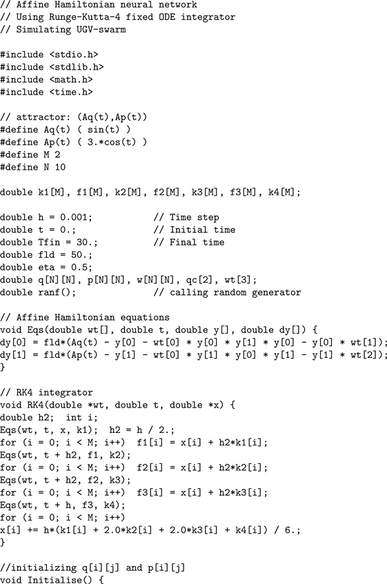
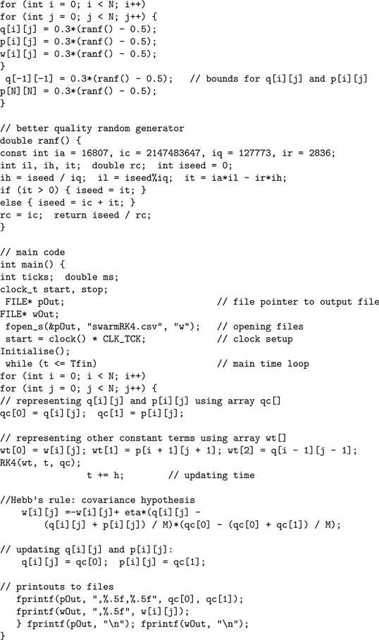
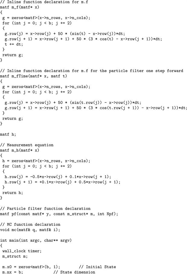
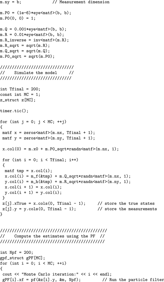
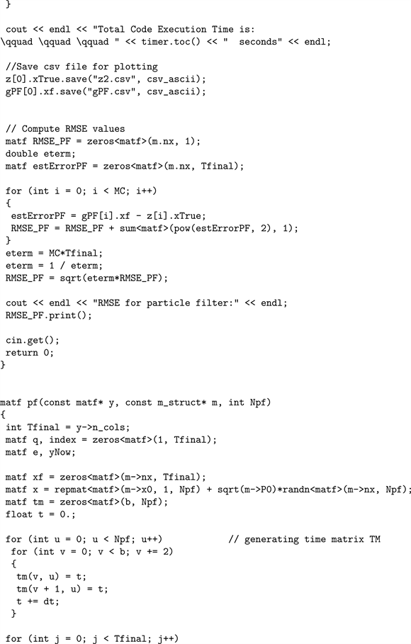
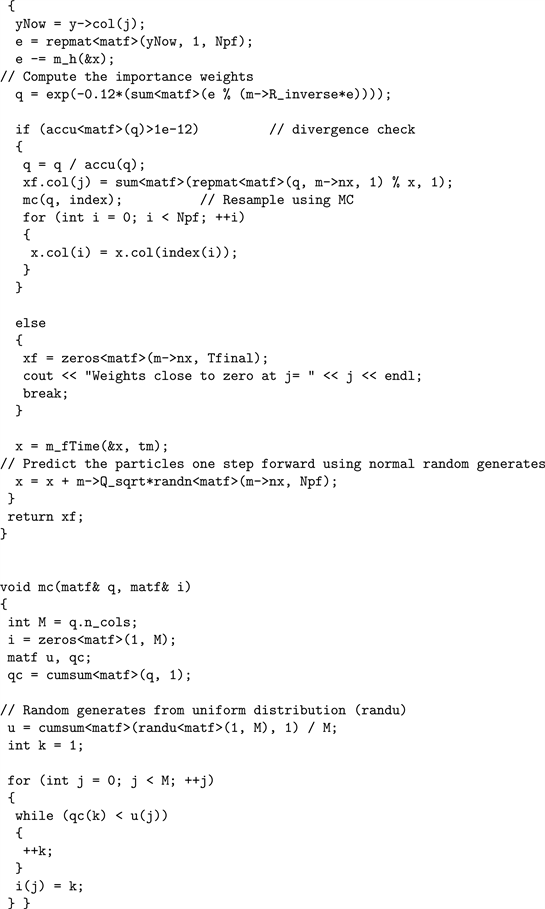
C++ code for the the Hamiltonian neural net is given in Appendix 1.1.
MathematicaÒ code
Dimensions:
Coordinates and momenta:

Figure 2. Adaptive control for a large fleet (a matrix) of 100 UGVs: time evolution of coordinates , where . As expected, we can see the exponential-type growth of coordinates together with their spreading from zero initial conditions. This plot is the simulation output of the recurrent activation dynamics given by Equations ((5), (6)) with Hebbian learning dynamics given by Equations ((11), (12)), starting from zero initial coordinates and momenta and random initial weights.

Figure 3. Adaptive control for a large fleet (a matrix) of 100 UGVs: time evolution of momenta . As expected, we can see the exponential-type decay of momenta together with their spreading, after the initial convergent growth from zero initial conditions. This plot is the simulation output from the same recurrent neural network as in Figure 2.

Figure 4. Adaptive control for a large fleet (a matrix) of 100 UGVs: time evolution of synaptic weights . As expected, we can see the converging behavior of the weights , starting from their initial random distribution. Simulating the same recurrent neural network from Figure 2.
Hyperbolic tangent activation functions:
Derivatives of activation functions:
Control inputs:
Affine Hamiltonians (nearest-neighbor coupling):
Attractor lines (figure-8 attractor):
Equations of motion:
Numerical solution:
Plots of coordinates:
Plots of momenta:
Plots of weights:
4. Estimation of an Autonomous Team of UGVs: High-Dimensional Bayesian Particle Filter
The second step in the nonlinear generalization of the Kalman servo is to replace the linear/Gaussian Kalman filter (4) with a general nonlinear/non-Gaussian Monte-Carlo filter, as follows.
4.1. Recursive Bayesian Filter
Recall that the celebrated Bayes rule gives the relation between the three basic conditional probabilities: i) a Prior (i.e., an initial degree-of-belief in event A, that is, Initial Odds), ii) Likelihood (i.e., a degree-of-belief in event B, given A, that is, a New Evidence); and Posterior: (i.e., a degree-of-belief in A, given B, that is, New Odds). Provided , Bayes rule reads:
(13)
In statistical settings, Bayes rule (13) can be rewritten as:
(14)
where is the prior probability density function (PDF) that the hypothesis H is true, is the likelhood PDF for the data D given a hypothesis H, is the posterior PDF that the hypothesis H is true given the data D, and the normalization constant: is the PDF for the data D averaged over all possible hypotheses .
When Bayes rule (13)-(14) is applied iteratively/recursively over signal distributions evolving in discrete time steps, in such a way that the Old Posterior becomes the New Prior and New Evidence is added, it becomes the recursive Bayesian filter, the formal origin of all Kalman and particle filters. The Bayesian filter can be applied to estimate the hidden state of a nonlinear dynamical system evolving in discrete time steps (e.g., a numerical solution of a system of ODEs, or discrete-time sampling measurements) in a recursive manner by processing a sequence of observations dependent on the state within a dynamic noise (either Gaussian, or non-Gaussian) measured as . The state dynamics and measurement, or the so-called state-space model (SSM) are usually given either by Kalman’s state Equation (1), or by its nonlinear generalization. Instead of the Kalman filter Equation (4) combined with the cost function (3), the Bayesian filter includes (see, e.g. [27] [28] ):
Time-update equation:
(15)
and
Measurement-update equation:
(16)
where is the normalizing constant, or partition function, defined by:
In the Bayesian filter (15)-(16), given the sequence of observations , the posterior fully defines the available information about the state of the system and the noisy environment―the filter propagates the posterior (embodying time and measurement updates for each iteration) across the nonlinear state-space model; therefore, it is the maximum a posteriori estimator of the system state. In a special case of a linear system and Gaussian environment, the filter (15)-(16) has optimal closed-form solution, which is the Kalman filter (4). However, in the general case of a nonlinear dynamics and/or the non-Gaussian environment, it is no longer feasible to search for closed-form solutions for the integrals in (15)-(16), so we are left with suboptimal, approximate, Monte Carlo solutions, called particle filters.
4.2. Sequential Monte Carlo Particle Filter
Now we consider a general, discrete-time, nonlinear, probabilistic SSM, defined by a Markov process , which is observed indirectly via a measurement process . This SSM consists of two probability density functions: dynamics and measurement . Formally, we have a system of nonlinear difference equations, given both in Bayesian probabilistic formulation (left-hand side) and nonlinear state-space formulation (right-hand side):
(17)
(18)
where and are the state and output vector-functions, and are non-Gaussian process and measurement noises and is a given non-Gaussian distribution. The state filtering problem means to recover information about the current state in (17) based on the available measurements in (18) (see, e.g. [29] ; for a recent review, see [30] and the references therein).
The principle solution to the nonlinear/non-Gaussian state filtering problem is provided by the following recursive Bayesian measurement and time update equations:
(19)
where
(20)
In a particular case of linear/Gaussian SSMs (17)-(18), the state filtering problem (19)-(20) has an optimal closed-form solution for the filter PDF , given by the Kalman filter (4). However, in the general case of nonlinear/non-Gaussian SSMs―such an optimal closed-form solution does not exist.
The general state filtering problem (19)-(20) associated with any nonlinear/ non-Gaussian SSMs (17)-(18) can be only numerically approximated using the sequential Monte Carlo (SMC) methods. The SMC-approximation to the filter PDF, denoted by , is an empirical distribution represented as a weighted sum of Dirac-delta functions:
(21)
where the samples are called particles (point-masses ‘spread out’ in the state space); each particle represents one possible system state and the corresponding weight assigns its probability. In this way defined particle filter (PF) plays the role of the Kalman filter for nonlinear/non-Gaussian SSMs. PF approximates the filter PDF using the SMC delta-approximation (21).
Briefly, a PF can be interpreted as a sequential application of the SMC technique called importance sampling (IS, see e.g. [31] ). Starting from the initial approximation: , at each time step the IS is used to approximate the filter PDF by using the recursive Bayesian Equations ((19), (20)) together with the already generated IS approximation of . The particles are sampled independently from some proposal distribution . To account for the discrepancy between the proposal distribution and the target distribution, the particles are assigned importance weights, given by the ratio between the target and the proposal: , where the weights are normalized to sum to one (for a recent technical review, see e.g., [30] ).
The IS proceeds in an inductive fashion:
which, inserted as an old/previous filter into the time-update Equation (20), gives a mixture distribution, approximating as:
(22)
Subsequent insertion of (22) as a predictor into the measurement-update Equation (19), gives the following approximation of the filter PDF:
which needs to be further approximated using the IS. The proposal density is pragmatically chosen as: . The N ancestor indices are resampled into a new set of particles which is subsequently used to propagate the particles to time t.
The final step is to assign the importance weights to the new particles as:
By evaluating for and normalizing the weights, we obtain a new set of weighted particles , constituting an empirical approximation of the filter PDF . Since these weighted particles can be used to iteratively approximate the filter PDF at all future times, this completes the PF-algorithm with an overall computational complexity of (as pioneered by [31] ; for more technical details, see e.g., [30] and the references therein).
We remark that the pinnacle of the PF-theory is the so-called Rao- Blackwellized (or, marginalized) PF, which is a special kind of factored PF, where the state-space dynamics (17) is split into a linear/Gaussian part and a nonlinear/non-Gaussian part, so that each particle has the optimal linear- Gaussian Kalman filter associated to it (see [32] - [40] ). However, in our case of highly nonlinear and adaptive dynamics, the use of Rao-Blackwellization does not give any advantage, while its mathematics is significantly heavier than in an ordinary PF.
5. Hamiltonian Servo Framework for General Control and Estimation
5Half continuous-time, half discrete-time.
The Hamiltonian servo system is our hybrid5 global control-estimation framework for a large team/fleet of UGVs (e.g., ), consisting of the following four components:
Adaptive Control, which is nonlinear and high-dimensional, defined by:
(23)
(24)
Measurement process, given in discrete-time, probabilistic and state-space Hamiltonian ( )-form:
(25)
where is a non-Gaussian measurement noise. Note that here we use the inverse dynamics (given coordinates, calculate velocities, accelerations and forces)―as a bridge between robot’s self-localization and control: measuring coordinates at discrete time steps t and from them calculating momenta and control forces ;
Bayesian recursions, given in discrete-time Hamiltonian ( )-form:
where
(26)
and
(27)
with IS weights:

Figure 5. Sample output of the Hamiltonian servo framework applied to a large fleet (a matrix) of 81 UGVs. As expected, the plot shows almost periodic time evolution of coordinates and momenta . Slight variation of both coordinates and momenta from the intended regular harmonic motion is due to adaptive control with initial random distribution of synaptic weights . This plot is the simulation output of the Hamiltonian neural network (23)-(24) and recurrent estimation (larger amplitudes, governed by the Bayesian particle filter (25)-(27)).
where bracketed superscripts label IS weights.
This Hamiltonian servo framework has been implemented in C++ language (using Visual Studio 2015; see Appendix 1.2). A sample simulation output of the servo system is given in Figure 5. The Figure demonstrates the basic stability and convergence of the servo system.
6. Conclusion
In this paper we have outlined a novel control and estimation framework called the Hamiltonian Servo system. The framework was shown to be a generalization of the Kalman Servo System. Using an example of a large team/fleet of 81 ( ) unmanned ground vehicles (UGVs), it was shown that the framework described provided the control and estimation as required. This approach encompassed a three tired system of adaptive control, measurement process and Bayesian recursive filtering which was demonstrated to enable control and estimation of multidimensional, non-linear and non-Gaussian systems.
Acknowledgements
The authors are grateful to Dr. Martin Oxenham, JOAD, DST Group, Australia for his constructive comments which have improved the quality of this paper.
Cite this paper
Ivancevic, V. and Pourbeik, P. (2017) Hamiltonian Servo: Control and Estimation of a Large Team of Autonomous Robotic Vehicles. Intelligent Control and Automation, 8, 175-197. https://doi.org/10.4236/ica.2017.84014
References
- 1. Hui, K.-P. and Pourbeik, P. (2011) OPAL—A Survivability-Oriented Approach to Management of Tactical Military Networks. IEEE MILCOM, 7-10 November 2011.
- 2. Nicholas, P., et al. (2016) Measuring the Operational Impact of Military SATCOM Degradation. Winter Simulation Conference (WSC), 11-14 December 2016.
- 3. Jormakha, J., et al. (2011) UAV-Based Sensor Networks for Future Force Warriors. International Journal of Advances in Telecommunications, 4, 58-71.
- 4. Offensive Swarm-Enabled Tactics (OFFSET). https://www.grants.gov/web/grants/view-opportunity.html?oppId=291825
- 5. Vukobratovic, M. and Potkonjak, V. (1982) Scientific Fundamentals of Robotics, Vol. 1, Dynamics of Manipulation Robots: Theory and Application. Springer, Berlin.
- 6. Vukobratovic, M. and Stokic, D. (1982) Scientific Fundamentals of Robotics, Vol. 2, Control of Manipulation Robots: Theory and Application. Springer, Berlin.
- 7. Vukobratovic, M. and Kircanski, M. (1985) Scientific Fundamentals of Robotics, Vol. 3, Kinematics and Trajectories Synthesis of Manipulation Robots. Springer, Berlin.
- 8. Vukobratovic, M. and Kircanski, N. (1985) Scientific Fundamentals of Robotics, Vol. 4, Real-Time Dynamics of Manipulation Robots. Springer, Berlin.
- 9. Vukobratovic, M., Stokic, D. and Kircanski, N. (1985) Scientific Fundamentals of Robotics, Vol. 5, Non-Adaptive and Adaptive Control of Manipulation Robots. Springer, Berlin.
- 10. Vukobratovic, M. and Potkonjak, V. (1985) Scientific Fundamentals of Robotics, Vol. 6, Applied Dynamics and CAD of Manipulation Robots. Springer, Berlin.
- 11. Ivancevic, V. and Ivancevic, T. (2006) Human-Like Biomechanics. Springer, Dordrecht.
- 12. ASIMO (2016) The Honda Humanoid Robot. http://world.honda.com/ASIMO/
- 13. Ivancevic, V.G. (2010) Nonlinear Complexity of Human Biodynamics Engine, Nonlin. Dynamics, 61, 123-139.
- 14. Durrant-Whyte, H. and Bailey, T. (2006) Simultaneous Localization and Mapping (SLAM): Part I. IEEE Robotics & Automation Magazine, 13, 99-110. https://doi.org/10.1109/MRA.2006.1638022
- 15. Wikipedia (2016) Simultaneous Localization and Mapping.
- 16. Montemerlo, M., Thrun, S., Koller, D. and Wegbreit, B. (2002) FastSLAM: A Factored Solution to the Simultaneous Localization and Mapping Problem.
- 17. Montemerlo, M., Thrun, S., Koller, D. and Wegbreit, B. (2003) FastSLAM 2.0: An Improved Particle Filtering Algorithm for Simultaneous Localization and Mapping That Provably Converges. Proceedings of IJCAI, 1151-1156.
- 18. Thrun, S., Montemerlo, M., Koller, D., Wegbreit, B., Nieto, J. and Nebot, E. (2004) FastSLAM: An Efficient Solution to the Simultaneous Localization and Mapping Problem with Unknown Data Association. Journal of Machine Learning Research, 1-48.
- 19. OpenSLAM (2016). https://www.openslam.org/
- 20. Kalman, R.E. (1960) A New Approach to Linear Filtering and Prediction Problems. Journal of Basic Engineering, 82, 34-45. https://doi.org/10.1115/1.3662552
- 21. Kalman, R.E. and Bucy, R.S. (1961) New Results in Linear Filtering and Prediction Theory. Journal of Basic Engineering, 96, 95-108. https://doi.org/10.1115/1.3658902
- 22. Kalman, R.E., Falb, P. and Arbib, M.A. (1969) Topics in Mathematical System Theory. McGraw Hill, New York.
- 23. Ivancevic, V. and Yue, Y. (2016) Hamiltonian Dynamics and Control of a Joint Autonomous Land-Air Operation. Nonlinear Dynamics, 84, 1853-1865. https://doi.org/10.1007/s11071-016-2610-y
- 24. Ivancevic, V. and Ivancevic, T. (2006) Geometrical Dynamics of Complex Systems. Springer, Dordrecht. https://doi.org/10.1007/1-4020-4545-X
- 25. Ivancevic, V. and Ivancevic, T. (2007) Neuro-Fuzzy Associative Machinery for Comprehensive Brain and Cognition Modelling. Springer, Berlin. https://doi.org/10.1007/978-3-540-48396-0
- 26. Kosko, B. (1992) Neural Networks and Fuzzy Systems, A Dynamical Systems Approach to Machine Intelligence. Prentice-Hall, New York.
- 27. Arulampalam, S., Maskell, S., Gordon, N. and Clapp, T. (2002) A Tutorial on Particle Filters for Online Nonlinear/Non-Gaussian Bayesian Tracking. IEEE Transactions on Signal Processing, 50, 174-188. https://doi.org/10.1109/78.978374
- 28. Ristic, B., Arulampalam, S. and Gordon, N. (2004) Beyond the Kalman Filter. Artech House.
- 29. Schön, T.B., Gustafsson, F. and Nordlund, P.-J. (2005) Marginalized Particle Filters for Mixed Linear/Nonlinear State-Space Models. IEEE Transactions on Signal Processing, 53, 2279-2289. https://doi.org/10.1109/TSP.2005.849151
- 30. Schön, T.B., Lindsten, F., Dahlin, J., et al. (2015) Sequential Monte Carlo Methods for System Identification. IFAC-PapersOnLine, 48, 775-786.
- 31. Gordon, N.J., Salmond, D.J. and Smith, A.F.M. (1993) Novel Approach to Nonlinear/Non-Gaussian Bayesian State Estimation. I Radar and Signal Processing, 140, 107-113.
- 32. Casella, G. and Robert, C.P. (1996) Rao-Blackwellisation of Sampling Schemes. Biometrika, 83, 81-94. https://doi.org/10.1093/biomet/83.1.81
- 33. Chen, R. and Liu, J.S. (2000) Mixture Kalman Filters. Journal of the Royal Statistical Society, 62, 493-508. https://doi.org/10.1111/1467-9868.00246
- 34. Doucet, A., Godsill, S.J. and Andrieu, C. (2000) On Sequential Monte Carlo Sampling Methods for Bayesian Filtering. Statistics and Computing, 10, 197-208. https://doi.org/10.1023/A:1008935410038
- 35. Doucet, A., Gordon, N. and Krishnamurthy, V. (2001) Particle Filters for State Estimation of Jump Markov Linear Systems. IEEE Transactions on Signal Processing, 49, 613-624. https://doi.org/10.1109/78.905890
- 36. Andrieu, C. and Doucet, A. (2002) Particle Filtering for Partially Observed Gaussian State Space Models. Journal of the Royal Statistical Society, 64, 827-836. https://doi.org/10.1111/1467-9868.00363
- 37. Schön, T., Gustafsson, F. and Nordlund, P.-J. (2003) Marginalized Particle Filters for Nonlinear State-Space Models. Tec. Report LiTH-ISY-R-2548, Linköping Univ.
- 38. Schön, T., Gustafsson, F. and Nordlund, P.-J. (2005) Marginalized Particle Filters for Mixed Linear/Nonlinear State-Space Models. IEEE Transactions on Signal Processing, 53, 2279-2289. https://doi.org/10.1109/TSP.2005.849151
- 39. Karlsson, R., Schön, T. and Gustafsson, F. (2005) Complexity Analysis of the Marginalized Particle Filter. IEEE Transactions on Signal Processing, 53, 4408-4411. https://doi.org/10.1109/TSP.2005.857061
- 40. Schön, T., Karlsson, R. and Gustafsson, F. (2006) The Marginalized Particle Filter in Practice. Aerospace Conference, 4-11 March 2006. https://doi.org/10.1109/AERO.2006.1655922
- 41. Wikipedia (2016) Armadillo (C++ Library).
Appendix: C++ Code
1.1. Affine Hamiltonian Neural Network
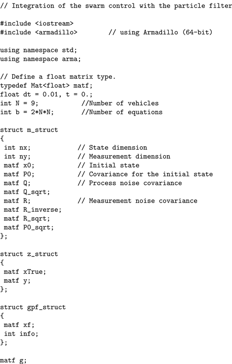
1.2. High-Dimensional Bayesian Particle Filter
The following C++ code uses the Armadillo matrix library [41] .
NOTES
1The acronym LQR means linear quadratic regulator.
2The acronym LQG means linear quadratic Gaussian.
3For simplicity, we are dealing with a square -matrix of UGV configurations. The whole approach works also for a rectangular -matrix, in which .