Circuits and Systems
Vol.09 No.11(2018), Article ID:88401,27 pages
10.4236/cs.2018.911017
Stabilization of Linear Multistage Amplifiers
J. Ladvánszky
Ericsson Telecom Hungary, Budapest, Hungary

Copyright © 2018 by author and Scientific Research Publishing Inc.
This work is licensed under the Creative Commons Attribution International License (CC BY 4.0).
http://creativecommons.org/licenses/by/4.0/


Received: July 25, 2018; Accepted: November 9, 2018; Published: November 12, 2018
ABSTRACT
In a given linear, multistage, cascaded amplifier [1] comprising passive coupling circuits and active two-ports alternatively, the problem is where in the amplifier the stabilizing circuit elements should be placed to eliminate instability, and of what type and value. Our investigations are based on a new recursive formula for the determinant of tridiagonal matrices. Relation of our results to the Stern stability factor has been obtained. A verification in numerical examples has also been provided.
Keywords:
Linear Multistage Amplifiers, Instability, Determinant, Tridiagonal Matrix, Stern Stability Factor

1. Introduction
Stability Theory is currently being revived in many disciplines. This is because of the novel results in chaotic systems and investigations into its robustness. In electrical engineering as well, these problems are of distinguished actuality in areas such as in automatics, control theory, and power electronics. However, in this study, we concentrate on electrical circuits.
In circuit theory, stability related problems are in close connection with appearance and application of feedback. These investigations were based on the observation that exotic phenomena are in close connection with singularities of the model. Characteristic of the early period is the graphical investigation of the loop gain. A later, well distinguished period can be described as a numeric investigation of stability that was often in connection with invariance properties. During the 1970s and 1980s, clarifications and multidimensional system investigations were performed. The above-mentioned renaissance began in the 1980s when Professor Chua and his colleagues, based on results from physics, started studying exotic phenomena in nonlinear circuits. Most important results of this period are the simplest circuit exhibiting chaotic phenomena and systematic investigation of chaotic behavior. More recent investigations are related to the utilization of chaotic circuits for information transfer. Besides, up to the most recent time, you can often find some novel results for describing chaotic circuit operation.
In Section 2, we overview some publications from the history above outlined that relate more closely to our work. Section 3 contains our result for the determinant of tridiagonal matrices. Section 4 describes stabilization of one stage amplifiers, with a numerical example. In Section 5, two stages are considered. In Section 6, factors of the determinant are related to the Stern stability factor. Generalization for more than two stages is provided in Section 7. In Section 8, numerical examples are found.
2. Overview
References in this Section are organized as linear, time invariant, then time variant, then nonlinear circuits. All references are provided in time order. Relation of the references to the proposed research is that all of them are founding papers of this topic.
An overview figure for the proposed research is in Figure 12.
1) The Section begins with results for linear, time-invariant, active circuits.
[2] discusses the Nyquist stability factor, a variant suggested by him based on Bode’s book, and the Gewertz stability conditions. For the Nyquist stability condition, he refers to the characteristic equation written for the loop gain. The three Gewertz conditions contain positivity of the real part of the input and output impedances and an inequality written for the inner loop gain. At the end of the article, variants that have been simplified for reciprocal, antireciprocal, and symmetric two-ports are also added.
[3] deals with passivity and stability. In the part that is devoted to passivity, study by Gewertz and stability conditions by Llewellyn are cited. He shows that a rearranged version of these stability conditions is also found in the famous study by the M.I.T. Laboratories. That article is also mentioned in which―without recognizing its significance―the formula of the Rollett stability condition was first published.
[4] gives a simple method for deriving the Llewellyn stability conditions. Simultaneous matching of two-ports at both ports―image parameters―are investigated. He concludes that this is possible only if the two-port is unconditionally stable, and the stability conditions are derived from the determinant of the quadratic equation that expresses matching. Maximum stable gain is also determined.
[5] deals with the maximum gain that can be achieved at a given degree of stability. He recognizes that a transistor that is not unilateral, can oscillate as a consequence of its inner feedback, even if there is no outer feedback. An inequality can be given for the inner loop gain that results in potential instability. From this point, it is obvious that a degree of stability needs to be introduced. By writing a power gain at the given value of the stability factor, and maximizing it with respect to the terminations, a maximum stable power gain is given. The article also contains an early approach to the gain-bandwidth problem. The article is concluded by comparison of gains of an amplifier with the given stability factor and proper number of stages with the same stability factor. [6] introduces the application of these results in the design of multistage, narrow-band amplifiers.
[7] generalizes for n-ports the theorem that a reciprocal two-port is stable if and only if it is passive.
[8] searches a stability condition that is immittance-invariant (substituting z, y, h or k parameters, its value remains unchanged). His stability factor is related to the reciprocal of the absolute value of the inner loop gain and the Stern stability factor, and it shows immittance invariance. Some theorems regarding the newly introduced stability factor are also presented.
[9] gives a stability condition that is immittance-invariant, invariant to the lossless terminations, change of input and output, and applicable to distinguish the regions of conditional and unconditional stability. For positive real input and output impedance or admittance, the newly introduced stability factor is between −1 and infinity. Between −1 and 1, the two-port is conditionally stable, above 1 it is unconditionally stable. He expresses power gain in a double-matched case in unconditionally stable region in terms of the stability factor, and he shows that it is immittance-invariant. Then, tending to 1 with the new stability factor (to the limit of conditional and unconditional stability), he gives the expression of the maximum stable gain and its invariance properties. The conclusion of his article is that the new stability factor is an inherent characteristic of a two-port, similar to the Mason invariant [10] .
[11] started with the statement that two multiports are simultaneously stable or unstable if all main minors of their Z matrix are identical. He applies this for such two-ports one of them being reciprocal. Previously, he proved that a passive reciprocal two-port is surely stable, and applying the two theorems, he obtained the Bolinder version of the Llewellyn stability conditions. He notes that this cannot be applied for more than two ports, because, in general, such Z matrices whose main minors are identical, cannot be constructed.
As stability and passivity are in so close connection, we give the reference that provides the most refined concept of passivity for linear multiports [12] . This proves that for passivity, it is a necessary and sufficient condition that the impedance matrix of the investigated multiport is a positive real matrix. Previously obtained theorems are analyzed and small inaccuracies are corrected.
[13] solves the problem of how much is the greatest power gain of the two-port, which has variable terminations and feedback, and if its Stern stability factor is fixed. Maximum gain is expressed with unilateral gain and stability factor, and the necessary feedback is given as well. [14] adds some new formulas for conjugate termination and variable or fixed feedback and the freely chosen or limited stability factor combined.
[15] criticizes [13] and [14] from two points of view. One of them is that variable feedback, keeping the other parameters constant, can only be realized by a circuit having infinitely high Mason invariant. The other one is that the formula used in the criticized articles for unilateral gain, is not identical to that of the Mason invariant, but it was obtained from conjugate matched gain by omitting the feedback. Besides those, formulas in the criticized articles are correct.
[16] investigates how to express the stability conditions by the scattering matrix. Similar to the Llewellyn conditions, three inequalities are given, and he tries to prove them in a similar manner that [11] followed. First two inequalities can be obtained without problems, but the third one is valid only for reciprocal circuits. He also gives the Rollett stability factor in terms of the S-parameters.
[17] gives a simplified form of the known stability conditions expressed in terms of S-parameters. The previously given three conditions are decreased to two: The Rollett stability factor must be greater than one and the determinant of the S matrix must be lower than one. Later, he analyzes the relation between its set of stability conditions to the previously published ones.
[18] publishes a theorem for the spectral radius and applies it to the stability investigations of linear circuits. Accordingly, spectral radius of a rational matrix of n variable is bounded above within the unit circle if and only if it is bounded above on its boundary. By application to the scattering matrix of multiports, he shows that stability of the investigated multiport can be decided by terminating the ports by uncoupled reactances. Therefore, a new proof of an old theorem is also given: A reciprocal multiport is stable if and only if it is rigorously passive.
[19] gives necessary and sufficient conditions of absolute stability (for arbitrary one-port terminations, in BIBO sense) of linear, time invariant multiports. Main learning from his study is that if we allow open or short circuit as termination, then the condition for the determinant of the Z matrix has to be completed by other conditions.
[20] deals with absolute stability of linear, time-invariant, distributed circuits. He means I/O stability. The so-called k-stability is introduced: He means stability with such terminations that first k1 ports are terminated by a k1 port, the next k2 port by a k2 port, and so on, with k1 + k2 + ∙∙∙ = n. This k-stability is connected to the stability concept known till date in such a manner that k1 = 1, k2 = 1, ∙∙∙ He gives for absolute stability a necessary and sufficient condition. He points out that k-stability in general is weaker than traditional stability.
For time invariant, lumped element circuits, stability is often investigated by the Hurwitz test. [21] gives necessary and sufficient conditions for an interval polynomial (whose coefficients are bounded above and below) being a Hurwitz polynomial. According to the cited Kharitonov stability condition, this can be deduced to the investigation of eight so-called limit polynomial. Limit polynomials can be obtained from the original one by substituting the coefficients according to some given rules and some further transformations.
[22] investigates the number of additional conditions that are needed for unconditional stability in addition to the Rollett stability factor. In his experiment, output of the two-port is terminated by a susceptance, and the locus of the input admittance is studied. He comes to the geometrical interpretation of the Rollett stability condition: The locus of the input admittance (a circle in this case) should not cross the imaginary axis. In his explanation, the additional conditions serve for deciding if the locus is at the right or left side of the axis. As the two sides are equivalent from the stability point of view, it is enough to fulfill one of the additional conditions. The same is valid for the scattering matrix description.
[23] [24] replaces the Rollett stability condition and the additional condition by one condition that is necessary and sufficient for unconditional stability. A new stability factor is introduced. Disadvantage of the result is that it is not invariant for the interchange of the input and output.
[25] investigates amplifiers containing many parallel-connected stages. The motivation is that in push-pull amplifiers, power transistors, and in microwave monolithic integrated circuits, such odd-mode oscillations have been observed that may cause damage of the device. Stability is investigated by the Nyquist test of the feedback loop. Results are verified by a circuit containing two or three devices.
2) As two examples, we continue with investigations of linear, time-variant circuits in time and complex frequency domain.
[26] publishes a basic result for stability of linear, time-variant circuits in time domain. The circuit is defined stable if it obtains a bounded output for a bounded input. This can only occur if the weight function of the circuit is absolute integrable. He notes that his result was motivated by a known result for stability of linear, time-invariant, sampled filters, and that a completely another approach is also known for his result.
[27] investigates the stability of linear, time-variant circuits. State-space approach is used. On stability, he means that for zero excitation, the answer is zero or an answer tending to zero (Ljapunov stability, asymptotic stability). Conditions for Ljapunov stability and asymptotic stability are given. He shows that his results are simpler and sharper than other results.
3) This overview is finished with some stability investigation results for nonlinear circuits.
[28] investigates the circle criterion [29] for periodically excited nonlinear circuits containing a linear, time-invariant circuit and a varactor diode. Asymptotic stability is considered: Answer must tend to a steady state with same period than that of the excitation. He shows that the investigated circuit may exhibit subharmonic oscillation. The circuit is stable if the voltage of the nonlinear part is bounded from above and below, and the locus of the quantity jωZ(jω) that is derived from the impedance Z(jω) of the linear subcircuit lies outside a circle that is derived from bounds.
Besides general stability conditions, several researchers publish conditions for specific nonlinear circuits [30] , [31] . Although practical value of such investigations is high, their validity is limited because of their circuit-specific nature. For this reason, general investigations that are applicable in practice have an especially high value.
In our early study [32] , we generalized the one-port stability condition given by [33] based on perturbation method, for the case of nonlinear two-ports. Generalization became possible because of introduction of two-port functions being described. Our investigations are based on an experience that for sinusoidal excited, tuned nonlinear amplifiers, instability occurs in the form of output with mixed amplitude and phase modulation. This modulation is considered as perturbation, and the stability investigation is the Routh-Hurwitz test of the perturbation transfer matrix. Applying for low-frequency, tuned amplifier, a circuit-specific stability condition is given, containing the feedback capacitance, characteristics of the nonlinear transfer, and the excitation level. This stability condition is in good agreement with the experimental fact that there is no instability for small excitations, instability appears at a critical level, and further increase of the excitation level results in stability again. The results were extended later for different input and output tuning and for synchronized oscillators.
This topic has other Hungarian-related results as well: Information transfer using chaotic circuits has been investigated by [34] .
3. Determinant of Tridiagonal Matrices
Let be a square matrix having nonzero entries only in the main and neighboring diagonals (tridiagonal matrix). The submatrix comprising the rows with serial number and columns is denoted as follows [35] [36] :
(1)
For determinant of , we introduce the notation .
Theorem 1. The determinant of the n × n matrix can be expressed as
(2)
where ai,k is the entry of in the ith row and kth column, and p is a positive integer with .
Meaning of (2) is illustrated in an example. Let n = 8 and p = 3. Submatrices in (2) are denoted by thick lines in Figure 1.
Proof: Full induction is applied where for n = 2 and p = 1 the following holds:
(3)
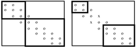
Figure 1. For the explanation of (2). Circles and crosses denote nonzero, the empty places denote zero entries. On the left, the first term of (2) is shown, whereas, on the right, the second one.
(4)
(5)
(6)
(7)
and we define
(8)
when the first row or column index is greater than the last one. If n = 2 and p = 2, then (2) holds as well.
We assume that the theorem is valid for n × n tridiagonal matrices when and prove that it holds for (n + 1) × (n + 1) if .
In the pth column, three entries are different from zero: ap-1,p, ap,p, ap+1,p. Thus
(9)
On the right side, all three determinants are determinants of n x n tridiagonal matrices; for that the assumption above holds:
(10)
From the tridiagonal property, it follows that
(11)
Therefore, (10) can be rewritten as
(12)
Now we apply the assumption for the second determinant on the right side of (9):
(13)
Because of the tridiagonal property, all entries with a difference of more than one between row and column indices is zero:
(14)
Thus (13) has a form of
(15)
Finally, the third determinant on the right side of (9) is expanded:
(16)
As
(17)
(16) is simplified as
(18)
Because of (9, 12, 15, 18):
(19)
On the right side of the last equation, we reformulate the second determinant, applying (2):
(20)
Because
(21)
and
(22)
(20) can be rewritten as
(23)
The last step is getting to know that the second and third term on the right side of (19) can be joined as
(24)
Based on (19, 23, 24):
(25)
and that is what we wanted to see. Pathologic cases (n < p) are trivial.
Explanation for Equation (25) is that it expresses the same as Equation (2) above and that we wanted to prove.
4. Stabilization of a One-Stage Amplifier
In this Section, Theorem 1 will be applied for stabilization of a one-port amplifier. The amplifier can be characterized in the following manner:
(26)
where the square matrix on the right is called the admittance matrix of the amplifier. Explanation for notations is found in Figure 1. The first and third blocks are coupling circuits, whereas, the second block is the active device (transistor). In building up the admittance matrix, reciprocity of the coupling circuits is exploited.
Transducer power gain is defined as
(27)
Power absorbed by the load is
(28)
where . Maximum generator power is
(29)
where . From (27)-(29):
(30)
The transducer power gain (30) is a function of the transfer impedance:
(31)
and that is obtained from (26) using Cramer’s rule. D is the determinant of the admittance matrix of the amplifier. The amplifier is unstable if
(32)
otherwise it is stable. Therefore,
Theorem 2. For stability of the amplifier, it is necessary that the zeroes of the determinant D are placed at the left half of the complex frequency plane. If the admittances in the nominator of (31) do not have right half plane poles, then the given condition is necessary and sufficient.
Proof: Now Theorem 1 will be applied for determining D. The admittance matrix of the amplifier is denoted by :
(33)
The determinants at the right side are written based on (26):
(34)
(35)
(36)
(37)
(38)
(39)
In (34), can be rewritten as a product:
(40)
In the second term on the right, we introduce a new notation. Output admittance of the first block in Figure 2, when the input is terminated by , is
(41)
Meaning of the new notation is clarified in Figure 3. With this notation:
(42)
Based on (35), similarly, can be expressed as a product:
(43)
where is the input admittance of block 3 in Figure 2 when its output is terminated by :
(44)
Utilizing (42) and (43), D in (33) can be written as follows:
(45)
The second term on the right side of (45) can be transformed:
(46)
where denotes output admittance of the block 2 in Figure 2 when its input is terminated by :
(47)
Thus, product decomposition of the determinant is

Figure 2. Block diagram of a one-stage, cascaded amplifier. Coupling circuits and the active element are denoted by 1, 3, and 2.

Figure 3. Physical meaning of the notation of (41).
(48)
Please recognize that the terms of the product decomposition correspond to the admittances at the connections of blocks as shown in Figure 4.
Theorem 3. Number of terms in the product decomposition of the determinant is equal to the number of interconnections in the amplifier. One of the terms is the admittance of interconnected ports, without any change in the amplifier. The other terms are also admittances at other interconnections, but with other ports short-circuited.
Proof: Figure 4 shows proof for one-stage amplifier. Extension for more stages are found in the next Sections.
Theorem 3 can be applied for finding circuit elements stabilizing the amplifier. For this, you have to recognize that a circuit element connected to the input of block 3 modifies only the third term of the determinant. The circuit element connected to the input of block two modifies the second and the third term, the circuit element at the input of block 1 modifies terms 1, 2, and 3, whereas the circuit element at the output of block three modifies terms 3 and 4. Hurwitz test of the terms specifies which term has to be modified and thus the place where it has to be connected is given.
The last statement is illustrated by an example. A one-stage amplifier is illustrated in Figure 5.
Determinant of the admittance matrix of the amplifier in Figure 5 has been determined in a half-symbolic form [37] , and a Hurwitz test has been performed. The Hurwitz test does not report instability in case of terms 1, 2, and 4. However, term 3 in (46) has a form of

Figure 4. Terms of the determinant are identical to interconnection admittances, with proper terminations at other ports.

Figure 5. Circuit diagram of a one-stage amplifier.
(49)
(50)
where p denotes complex frequency. A(p) is not a Hurwitz polynomial because the sign of the fifth order term is different from others. For this reason, a stabilizing element to be connected at the input of the block 3 is needed. Let it be a resistor whose element value is determined so that the Rollett stability factor equals to one at the edge of the passband. The stabilized amplifier with its characteristic before and after stabilization are shown in Figures 6-8.
In Figure 7 and Figure 8, the Rollett stability factor, that is, the determinant of the scattering matrix of the amplifier (that appears in the Woods stability condition) are denoted by K and Det, respectively. Gain is smaller in the stabilized

Figure 6. The stabilized amplifier.

Figure 7. Characteristics of the amplifier before stabilization.

Figure 8. Characteristics of the amplifier after stabilization.
amplifier, of course. Det < 1 in both cases, satisfying the stability condition regarding the determinant. Before stabilization, K < 1 at the lower edge of the passband, hurting the stability condition, and K > 1 in the whole passband, after stabilization.
5. Two-Stage Amplifier
A two-stage cascaded amplifier can be characterized as follows:
(51)
For determining the power gain, we have to formulate the transfer impedance as it can be seen from (30):
(52)
where D denotes now the determinant of the 6 × 6 admittance matrix in (51). In the following, we calculate the product decomposition of D. If Theorem 1 is applied for n = 6 and p = 2, then n = 4 and p = 2, and the result is rearranged as in the previous Section; we arrive at the following expression:
(53)
where the following notations have been introduced:
(54)
the output admittance of block 1 when its input is terminated by ,
(55)
the input admittance of block 5 when its output is terminated by ,
(56)
the output admittance of block 2 when its input is terminated by ,
(57)
the input admittance of block 4 when its output is terminated by ,
(58)
the output admittance of block 3 when its input is terminated by .
Terms of D in (53) are identical to the admittances in Figure 9 at the dashed lines.
Thus, as it is written in the previous Section, Hurwitz test of the terms in (53) can be applied for determining the place of the stabilizing circuit elements.
Product decomposition of the determinant is not unique. As a consequence, a specific stabilization problem can be solved at least two ways. Solutions for one- and two-stage amplifiers are summarized in Table 1(a) and Table 1(b) and Table 2(a) and Table 2(b).
Table 1(a) and Table 1(b) contain examples for the relation of non-Hurwitz terms and the places for stabilization for one-stage amplifiers. Those ports that modify the terms according to the given columns are denoted by X. Thus, for example, if the first term of the determinant is non-Hurwitz, then that term can be modified by the circuit element connected to port 1, 2, or 3. For stabilization
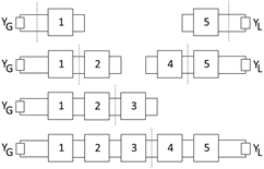
Figure 9. Terms of the determinant of the admittance matrix of the two-stage amplifier.
(a)  (b)
(b)
Table 1. Examples for one-stage amplifiers.
(a) (b)
Table 2. (a) Examples for the relation of non-Hurwitz terms and the places for stabilization; (b) More examples for the relation of non-Hurwitz terms and the places for stabilization.
of the amplifier, we exploit that there are ports where, if a stabilizing circuit element is connected, then not all terms are modified. For example, a circuit element connected to port 1, does not influence term 2, 3, or 4.
The difference between Table 1(a) and Table 1(b) is the “center” term in the product decomposition.
6. Relation to the Stern Stability Factor
Instability of the investigated amplifiers are caused by the feedback inside the active elements. Instability can also be traced by investigating the real part of the terms of the determinant. Therefore, it is interesting to investigate the ratio of the real part of the terms with and without feedback. For example, in case of a two-stage amplifier, the third term in (53) is:
(59)
and the value of without the feedback of the active element (block 2) is
(60)
The above-mentioned ratio is
(61)
Physical interpretation of the terms in d3 is given in Figure 10.
Relation between the Stern stability factor and the minimum of d3 is
(62)
where S3 is the Stern stability factor of the circuit in the upper right corner of Figure 10.
We denote by y a term of the determinant that is identical to the admittance at the load side port of an active element. The following idea is valid also for generator side admittance; thus, a full generalization of (62) is made. Denote by y0 the value of y when the feedback is omitted. Let us denote by YG and YL the terminating admittances according to Figure 11.
Let
(63)
and let S denote the Stern stability factor of the amplifier in Figure 11.
Theorem 4.
(64)
Proof: First we recognize that d depends on GG, GL, and BG, but it does not depend on BL ( ). For this reason, to keep the power gain constant, we keep GG, GL constant and we seek for the minimum as a function of BG. Then we compare the expression for dmin to the definition of the Stern stability factor.
Applying the notations of Figure 11, y can be expressed as follows:
(65)
When determining the real part of y, we introduce the following notations:
(66)
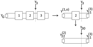
Figure 10. Physical meaning of the quantities in (61).

Figure 11. An amplifier operating between terminating admittances YG and YL.
Real and imaginary parts of the admittance matrix entries are denoted by G and B, respectively, properly indexed.
(67)
Let
(68)
(69)
(70)
Real part of y is the following:
(71)
and really, g does not depend on BL. We seek gmin as a function of BG, therefore, we have to solve the following equation:
(72)
or in more detailed form,
(73)
The solution is
(74)
Minimum of g is found by substituting (74) into (71):
(75)
If the active element does not have inner feedback, then M = N = 0, thus, from (71):
(76)
From (75) and (76):
(77)
The definition of the Stern stability factor [18] is
(78)
Therefore, the relation between the Stern stability factor and dmin can be expressed as
(79)
The Stern stability condition is
(80)
Thus from (79) and (80):
(81)
as expected.
Note that the proof contains more to learn. Using the results above, (3) can be proven in a simple way, as follows. For stability, terms of the determinant must not have roots in the closed right half plane. From this and from passivity of y0, (81) follows at the jω axis. From (81) and (79), (80) follows, and finally, from (80) and (78) results in (3).
We also note that for a two-stage amplifier, not considering feedback in active elements does not influence the terms 1, 2, 5, and 6, thus if i = 1, 2, 5, or 6. In these cases, Theorem 2 is useless. On the contrary, in a multistage amplifier, Theorem 2 holds for all terms that are modified when the feedback of the active elements is omitted.
7. A Multistage Amplifier
In this Section, the stabilization method introduced in the previous Sections is generalized. Generalization is based on the fact that in the recursive formula for the determinant of tridiagonal matrices, direction of recursion can be changed once.
Theorem 5.
If is an n × n tridiagonal matrix, and m is a positive integer, , then the determinant of can be expressed as follows:
(82)
(83)
(84)
(85)
(86)
(87)
Proof: We will see that the Theorem is valid for m = n − 1, then we assume it holds for m and prove that it holds for m − 1 as well.
(88)
(89)
(90)
The n-1th and nth terms in detail are as follows:
(91)
(92)
Then the product of these two terms is rewritten as
(93)
Comparing this with (85), we can see that the Theorem is valid for m = n − 1 as we wanted. Now we assume it is valid for m, and terms m − 1 and m are written as
(94)
if , and
(95)
if .
Similarly, as in (93), we rewrite the product of these two terms:
(96)
If in (82)-(87), we leave all terms unchanged except terms m − 1 and m, and at the place of these terms (96) is written, then the theorem is proven.
Now we apply Theorem 5 for the admittance matrix of an n-stage amplifier. Figure 12 shows the block diagram of an n-stage amplifier. Odd and even numbered blocks denote the coupling circuits and the active elements, respectively.
This amplifier can be characterized as follows:
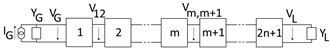
Figure 12. The block diagram of an n-stage amplifier. Odd numbered blocks are coupling circuits, even numbered ones are active elements.
(97)
Applying Theorem 5 for the admittance matrix in (97), product decomposition of the determinant is the following:
(98)
where the following notations were introduced: Output admittance of block 1 when the input termination is :
(99)
Output admittance of block m when the input termination is :
(100)
Input admittance of block m + 1 when its output is terminated by :
(101)
Input admittance of block 2n + 1 when its output is terminated by :
(102)
Terms of (98) have physical meaning. In case of n-stage amplifier, there are 2n + 2 terms, where 2n + 1 terms are equal to the admittance at a port interconnection, when another interconnection is short-circuited. In case of the remaining term, the short circuit must not be applied. Physical meaning of the terms is summarized in Figure 13. With this step, proof of Theorem 3 is completed.

Figure 13. Terms of the determinant in the product decomposition (98) are equal to the admittances that can be measured at dashed lines.
Equation (98) can be applied for stabilization of n-stage amplifiers as it was described in the previous Sections. Note that the fact that coupling circuits and active elements follow each other alternatively was not deeply exploited. Therefore, our results can be reasonably applied for arbitrary order of components.
It would result in further simplification if the direction of recursion in (82)-(87) could be altered once more. But we can see easily that this is not possible. The reason is that we exploited in (82)-(87) the property of (88)-(90), that is, that terms do not depend on other terms with higher serial number. On the contrary, the mth term in (85) depends on terms m − 1 and m + 1, and all terms of lower serial number depend on the previous ones, whereas those of higher serial number depend on the next terms. Therefore, recursion can be altered only once.
8. Examples
Next, you can find a simple example for illustration that product decomposition of the determinant can be utilized for characterization of stability based on circuit element values.
Product decomposition in (48) is applied here for a one-stage field-effect transistor (FET) amplifier. Circuit schematics is shown in Figure 14.
According to Theorem 3, the determinant is a product of four terms. Roots of first, second, and fourth terms lie in the left half plane. Thus, stability of the amplifier depends on the third term. Regarding (48), the third term can be expressed as follows:
(103)
where p stands for the complex frequency. When , the above expression is simplified as
(104)
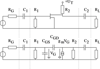
Figure 14. One-stage RC coupled FET amplifier schematics and its model. Parts of the circuit are separated by dashed lines.
Thus, the stability of the amplifier is determined by the real part of the roots of the following equation:
(105)
Recognize that the right side of (105) is the determinant of the admittance matrix of the FET model completed with resistive elements. If the FET does not have inner feedback, then the second term would appear, and the real part of the roots is always negative. The learning from this example is that our method is very efficient in characterizing stability.
Next, we investigate a two-stage amplifier designed for the 0.5 - 2.5 GHz band. The amplifier does not meet the stability conditions. We analyze the terms of the determinant and we obtain a possible way for stabilization.
Schematics of the amplifier is shown in Figure 15. Characteristics are shown in Figure 16 and Figure 17. The stability condition K > 1 is hurt, where K is the Rollett stability factor.

Figure 15. Schematics of the investigated two-stage amplifier.

Figure 16. S21 as a function of frequency.
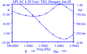
Figure 17. The Rollett stability factor K and the determinant of the scattering matrix of the amplifier.
Recognize that we have to separate the parts of the amplifier differently than what is shown in Figure 15. As the blocks 1 and 3 in Figure 15 have poles at the jω axis, they hurt the conditions of Theorem 2. New blocks are shown in Figure 18.
Now (98) applies for seven blocks; thus, the number of terms is 8. The circuit is cut between blocks 4 and 5; thus m = 4. In the product decomposition, obviously terms 1, 2, and 8 do not exhibit instability. Numerators of the other terms are determined in half-symbolic form [17] . Coefficient of the lowest power term is normalized to 1.
(106)
(107)
(108)
(109)
(110)
It is obvious that in case of A7 there is no stability problem. In case of A3, A4, and A7, the coefficients and all Hurwitz determinants [34] are positive. Therefore, we have stability problem only in case of A5. The problem is solved by R5 that is connected between blocks 4 and 5. R5 modifies only term 5; therefore, no more stabilizing elements are necessary. To have all coefficients of A5 positive, kohm resistor is needed. Circuit schematics and characteristics are given in Figures 19-21.
9. Conclusions
Our problem was to determine places where stabilizing elements could be connected in a linear multistage cascaded amplifier. We showed that the problem
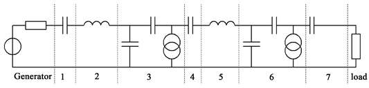
Figure 18. Blocks of the amplifier modified.

Figure 19. Schematics of the two-stage amplifier after stabilization.

Figure 20. S21 as a function of frequency.
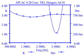
Figure 21. The Rollett stability factor K and the determinant of the scattering matrix of the amplifier.
leads to the product decomposition of the determinant of the admittance matrix of the amplifier. For this reason, we obtained identities for the determinants of tridiagonal matrices, and we applied them for our problem. We showed that Hurwitz test of the terms of the determinant provides a possibility for finding places for the stabilizing elements. We proved that the terms of the determinant are in close connection with the Stern stability factor.
In practice, it is convenient to connect stabilizing elements with ports of blocks of the amplifier. For this reason, we solved our problem based on the admittance matrix description of the amplifier. Other formalisms, for example, impedance matrix, can also be used and that leads to stabilizing elements in series with the ports.
Stability can also be provided using feedback. Using low-loss circuit elements for the feedback, maximum stable gain can be approached. In our method, resulting stabilized gain is smaller than that, but in return, we have a conveniently applicable procedure, and the stabilizing elements can be inserted at the ready amplifier.
The method is not directly applicable for stabilizing distributed circuits. For our method, lumped-element model is necessary.
The product decomposition introduced is not unique. It depends on selecting the value of m in (98). We showed in examples that the method can be efficiently applied in writing circuit-specific stability conditions, and that transfer admittances of the blocks must not have right half plane poles.
Acknowledgements
With this article, the author remembers his former first master, Dr. A. Baranyi, with whom these investigations were started. We have received the problem from Prof. L. Pap, and we are grateful for that. The author is grateful to Prof. P. Rózsa, his former examiner for the PhD degree, who checked that turning the direction of recursion is really a new result. Prof. T. Berceli, Dr. E. Simonyi, V. Beskid, A. Bartus, and Dr. B. Kovács are also acknowledged for providing the author the best possible research conditions that were necessary for writing this article.
Conflicts of Interest
The authors declare no conflicts of interest regarding the publication of this paper.
Cite this paper
Ladvánszky, J. (2018) Stabilization of Linear Multistage Amplifiers. Circuits and Systems, 9, 169-195. https://doi.org/10.4236/cs.2018.911017
References
- 1. Ladvánszky, J. (1999) On the Stability of Multistage Amplifiers. Proceedings of the European Conference on Circuit Theory and Design, ECCTD’99, Stresa, August 29-September 2 1999, 635-638.
- 2. Llewellyn, F.B. (1952) Some Fundamental Properties of Transmission Systems. Proceedings of the IRE, 271-283.
- 3. FolkeBolinder, E. (1957) Survey of Some Properties of Linear Networks. IRE Transactions on Circuit Theory, 70-78.
- 4. Karp, M.A. (1957) On Gain and Stability. IRE Transactions on Circuit Theory, 339-340.
- 5. Stern, A.P. (1957) Stability and Power Gain of Tuned Transistor Amplifiers. Proceedings of the IRE, 335-343.
- 6. Lim, M. (1960) Power Gain and Stability of Multistage, Narrow-Band Amplifiers Employing Nonunilateral Electron Devices. IRE Transactions on Circuit Theory, 158-166.
- 7. Youla, D. (1959) A Stability Characterization of the Reciprocal Linear Passive N Port. Proceedings of the IRE, 1150-1151.
- 8. Venkateswaran, S. (1961) An Invariant Stability Factor and Its Physical Significance. IEEE Monograph.
- 9. Rollett, J.M. (1962) Stability and Power Gain Invariants of Linear Twoports. IRE Transactions on Circuit Theory, 29-32.
- 10. Mason, S.J. (1954) Power Gain in Feedback Amplifiers. IRE Transactions on Circuit Theory, CT-1, 20-25. https://doi.org/10.1109/TCT.1954.1083579
- 11. Youla, D. (1960) A Note on the Stability of Linear, Nonreciprocal n-Ports. 121-122.
- 12. Kuo, Y.L. (1968) A Note on the n-Port Passivity Criterion. IEEE Transactions on Circuit Theory, 74-76. https://doi.org/10.1109/TCT.1968.1082767
- 13. Scanlan, J.O. and Singleton, J.S. (1962) The Gain and Stability of Linear Two-Port Amplifiers. IRE Transactions on Circuit Theory, 240-246.
- 14. Scanlan, J.O. and Singleton, J.S. (1962) Two-Ports-Maximum Gain for a Given Stability Factor. IRE Transactions on Circuit Theory, 428-429.
- 15. Singhakowinta, A. and Boothroyd, A.R. (1964) On Linear Two-Port Amplifiers. IRE Transactions on Circuit Theory, 169.
- 16. Ku, W.H. (1966) Unilateral Gain and Stability Criterion of Active Two-Ports in Terms of Scattering Parameters. Proceedings of the IEEE, 54, 1617-1618. https://doi.org/10.1109/PROC.1966.5229
- 17. Woods, D. (1976) Reappraisal of the Unconditional Stability Criteria for Active 2-Port Networks in Terms of S Parameters. IEEE Transactions on Circuits and Systems, 23, 73-81. https://doi.org/10.1109/TCS.1976.1084179
- 18. Youla, D.C. (1980) A Maximum Modulus Theorem for Spectral Radius and Absolutely Stable Amplifiers. IEEE Transactions on Circuits and Systems, 27, 1274-1276. https://doi.org/10.1109/TCS.1980.1084757
- 19. Zeheb, E. and Walach, E. (1981) Necessary and Sufficient Conditions for Absolute Stability of Linear n-Ports. Circuit Theory and Applications, 9, 311-330. https://doi.org/10.1002/cta.4490090306
- 20. Bhaya, A. and Desoer, C.A. (1985) Absolute k-Stability of Linear Distributed n-Ports. IEEE Transactions on Circuits and Systems, 32, 625-634. https://doi.org/10.1109/TCS.1985.1085775
- 21. Bose, N.K. and Shi, Y.Q. (1987) A Simple General Proof of Kharitonov’s Generalized Stability Criterion. IEEE Transactions on Circuits and Systems, 34, 1233-1237. https://doi.org/10.1109/TCS.1987.1086055
- 22. Meys, R.P. (1990) Review and Discussion of Stability Criteria for Linear 2-Ports. IEEE Transactions on Circuits and Systems, 37, 1450-1452. https://doi.org/10.1109/31.62423
- 23. Edwards, M.L. and Sinsky, J.H. (1992) A Single Stability Parameter for Linear 2-Port Circuits. IEEE MTT-S Digest, 885-888.
- 24. Edwards, M.L. and Sinsky, J.H. (1992) A New Criterion for Linear 2-Port Stability Using a Single Geometrically Derived Parameter. IEEE Transactions on Microwave Theory and Techniques, 40, 2303-2311. https://doi.org/10.1109/22.179894
- 25. Ohtomo, M. (1993) Stability Analysis and Numerical Simulation of Multidevice Amplifiers. IEEE Transactions on Microwave Theory and Techniques, 41, 983-991.
- 26. Youla, D.C. (1963) On the Stability of Linear Systems. IEEE Transactions on Circuit Theory, 276-279. https://doi.org/10.1109/TCT.1963.1082108
- 27. Kuh, E.S. (1965) Stability of Linear Time-Varying Networks—The State Space Approach. IEEE Transactions on Circuit Theory, 12, 150-157. https://doi.org/10.1109/TCT.1965.1082427
- 28. Trick, T.N. (1969) Asymptotic Stability of a Class of Networks Containing a Nonlinear Time-Varying Capacitor and Periodic Inputs. IEEE Transactions on Circuit Theory, 16, 217-219. https://doi.org/10.1109/TCT.1969.1082929
- 29. Sandberg, I.W. (1965) Some Results on the Theory of Physical Systems Governed by Nonlinear Functional Equations. Bell System Technical Journal, 44, 871-898. https://doi.org/10.1002/j.1538-7305.1965.tb04161.x
- 30. Choma, J. (1972) Frequency Domain Stability Criteria for Large-Signal Tuned COmmon-Base Amplifiers. IEEE Transactions on Circuit Theory, 19, 265-270. https://doi.org/10.1109/TCT.1972.1083460
- 31. Vidkjaer, J. (1976) Instabilities in RF-Power Amplifiers Caused by a Self-Oscillation in the Transistor Bias Network. IEEE Journal of Solid-State Circuits, 11, 703-712. https://doi.org/10.1109/JSSC.1976.1050801
- 32. Baranyi, A. and Ladvánszky, J. (1984) On the Stability of Non-Linear Two-Port Amplifiers. Circuit Theory and Applications, 12, 123-131. https://doi.org/10.1002/cta.4490120206
- 33. Belevitch, V. (1959) Théorie des circuits non-linéariesen régime alternatif. Uystpruyst, Louvain.
- 34. Kolumbán, G. and Frigyik, B. (1999) Robust Chaotic Communications without Syncronization. Proceedings of the European Conference on Circuit Theory and Design, Stresa, 29 August-2 September 1999.
- 35. Rózsa, P. (1991) Linear Algebra and Its Applications. In Hungarian, Budapest, Tankönykiadó.
- 36. Gantmacher (1959) Theory of Matrices. Chelsea.
- 37. DesignSoft Inc. (1995) TINA 3.0—Toolkit for Interactive Network Analysis. User’s Guide.