Circuits and Systems
Vol.07 No.11(2016), Article ID:70380,17 pages
10.4236/cs.2016.711292
Design of Soft Computing Based Optimal PI Controller for Greenhouse System
A. Manonmani1, T. Thyagarajan2, S. Sutha2, V. Gayathri2
1Department of Electronics and Instrumentation Engineering, Saveetha Engineering College, Chennai, India
2Department of Instrumentation Engineering, MIT Campus, Anna University, Chennai, India

Copyright © 2016 by authors and Scientific Research Publishing Inc.
This work is licensed under the Creative Commons Attribution International License (CC BY 4.0).
http://creativecommons.org/licenses/by/4.0/


Received: May 6, 2016; Accepted: May 18, 2016; Published: September 6, 2016
ABSTRACT
Greenhouse system (GHS) is the worldwide fastest growing phenomenon in agricultural sector. Greenhouse models are essential for improving control efficiencies. The Relative Gain Analysis (RGA) reveals that the GHS control is complex due to 1) high nonlinear interactions between the biological subsystem and the physical subsystem and 2) strong coupling between the process variables such as temperature and humidity. In this paper, a decoupled linear cooling model has been developed using a feedback-feed forward linearization technique. Further, based on the model developed Internal Model Control (IMC) based Proportional Integrator (PI) controller parameters are optimized using Genetic Algorithm (GA) and Particle Swarm Optimization (PSO) to achieve minimum Integral Square Error (ISE). The closed loop control is carried out using the above control schemes for set-point change and disturbance rejection. Finally, closed loop servo and servo-regulatory responses of GHS are compared quantitatively as well as qualitatively. The results implicate that IMC based PI controller using PSO provides better performance than the IMC based PI controller using GA. Also, it is observed that the disturbance introduced in one loop will not affect the other loop due to feedback-feed forward linearization and decoupling. Such a control scheme used for GHS would result in better yield in production of crops such as tomato, lettuce and broccoli.
Keywords:
Greenhouse System, Feedback-Feed Forward Linearization and Decoupling, IMC Based PI Controller, Genetic Algorithm, Particle Swarm Optimization, Nonlinear System

1. Introduction
The GHS consists of highly coupled subsystems: the greenhouse climate and the greenhouse crop. The greenhouse control problem is to create a favorable environment for the crop in order to reach predetermined results for high yield, high quality and low costs. It is very difficult to control the GHS in practice, due to the complexity of the greenhouse environments such as high non-linearity, strong coupling between Multi-Input Multi-Output (MIMO) systems.
There are several models available for the GHS. Some of them use white box (first principle model) [1] [2] and others use black box model [3] - [5] . The best benchmark climate model is presented by Albright et al. [1] for controlling the temperature and humidity. A model based on feedback-feed forward compensation technique used for linearization, decoupling and disturbance compensation is presented in [1] [2] . Multi-ob- jective optimization of greenhouse system using evolutionary algorithm is given in [6] .
In this paper, a model of nonlinear thermodynamic laws between numerous system variables affecting the greenhouse climate is formulated and a feedback-feed forward approach to system linearization and decoupling is done. A conventional IMC based PI controller is designed based on the model. The IMC-PI controller parameters are optimized using Genetic Algorithm (GA) and Particle Swarm Optimization (PSO). The performance measures are compared for servo and servo-regulatory systems.
This paper is organized as follows: Section 2 briefs about a greenhouse system model. The control schemes are explained in Section 3 followed by closed loop analysis in Section 4. Section 5 gives details about the quantitative comparison. Finally, conclusions are presented in Section 6.
2. Greenhouse System Model
2.1. Description of Greenhouse Model
The three models for the greenhouse system include: cooling model, heating model and ventilating model. Ventilation is one of the most important components for a successful greenhouse. If there is no proper ventilation, greenhouses and their plants become prone to problems. The main purpose of ventilation is to regulate the temperature at the optimum level, to ensure movement of air and also to ensure the supply of fresh air for photosynthesis and plant respiration. Heating model is essential, when the inside temperature of the greenhouse is very low during winter climate and at night time. Whereas, cooling model is required when the outside temperature is very high which may affect the plants during the summer mode at day time. The functional block diagram of GHS is shown in Figure 1.
A simple greenhouse heating-cooling-ventilating model can be obtained (as given in Equation (1)) by considering the diff erential equations, which govern sensible and latent heat, as well as water balances on the interior volume [5] [6] :
 (1)
(1)
where
Tin/Tout: Indoor/outdoor temperature (˚C)
Hin/Hout: Interior/exterior humidity (g[H2O/kg[dry air])
Qheater: Heat provide by the greenhouse heater (W)
Qfog: Water capacity of fog system (g/s)
VR: Ventilation rate (m3/s)
The greenhouse system model parameters are shown in the Table 1.
In general, the operating conditions of the ventilation/cooling process are rather dominated by solar radiation alone (i.e. ), hence
  can be neglected. Suppose that
 ,
,  ,
,  and
and . The control variables can be normalized as follows:
 ,
,  and
and .
.
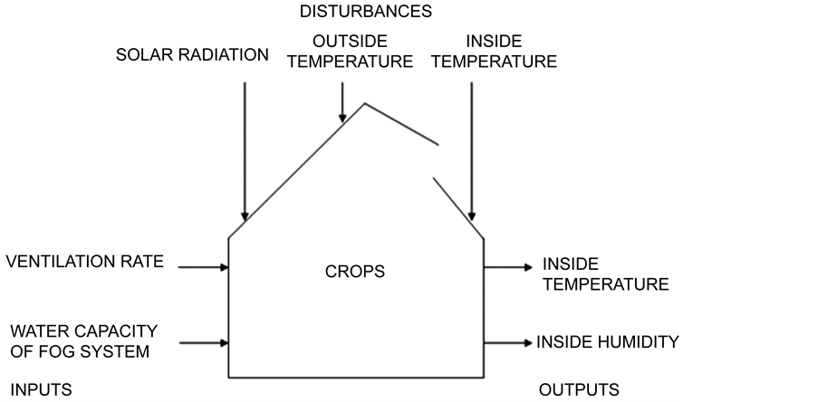
Figure 1. Block diagram representing greenhouse system.

Table 1. Greenhouse system model parameters.
In summer mode operation, Qheater is set to zero. The climate model provided have two variables to be regulated, namely the indoor air temperature (Tin) and the humidity ratio (Hin), through the process of ventilation VR,%(t) and fogging QR,%(t). After normalizing the control variables, the differential equation for cooling model for greenhouse system is re-written as given in Equation (2)
 (2)
(2)
In order to express the GHS in state-space form, the inside temperature and absolute humidity are defined as the dynamic state variables, x1(t) and x2(t), respectively; the ventilation rate and the water capacity of the fog system as the control (actuator) variables, u1(t) and u2(t), respectively; the intercepted solar radiant energy, the outside temperature, and the outside absolute humidity as the disturbances, vi(t), i = 1, 2, 3. The Equation (2) can alternatively be written in the following state-space form:
 (3)
(3)
 (4)
(4)
Relative Gain Array Analysis
From the state-space form the values of A, B and C is given by:


In this case relative gains are positive values. If 0 < λ11 < 1, then an interactions exists. From the interaction analysis it is found that y1 is paired withu1 and y2 is paired withu2 to form two loops with minimum interaction. However, the disturbances at one loop will affect responses of other loop due to coupling. Hence, decoupling is necessary for GHS. The feedback-feed forward linearization technique is used for decoupling is discussed in the subsequent section.
2.2. Feedback-Feed Forward Linearization and Decoupling
One method for linearization and decoupling for systems with external disturbances is presented in [2] [3] which is based on the feedback-feed forward linearization technique proposed by Isidori [4] . In the particular case of GHS model expressed in Equations (3) and (4), the feedback-feed forward linearization and decoupling procedure described above is followed and compensator is designed. The compensator that delivers the process input control variables u(u1, u2), has the form given in Equations (5) and (6).
 (5)
(5)
 (6)
(6)
where Q(t) must be anon-zero quantity.
 (7)
(7)
where,
 temperature change;
 humidity change.
The transfer functions derived from the linearized and decoupled GHS are as given in Equations (8) and (9)
 (8)
(8)
 (9)
(9)
3. Design of IMC Based PI Controller
3.1. Conventional IMC-PI Controller
In the Internal Model Control (IMC) formulation, the controller, q(s), is based directly on that part of the process transfer function which can be inverted. The IMC formulation generally results in only one tuning parameter, the closed loop time constant (λ, the IMC filter factor). The PI tuning parameters are then becomes a function of this closed-loop time constant. The selection of the closed-loop time constant is directly related to the robustness (sensitivity to model error) of the closed-loop system.
The feedback controller  contains the internal model
  and internal model controller, q(s). Now, the IMC design procedure can be used to design a standard feedback controller. The standard feedback controller is a function of the internal model,
  and internal model controller, q(s) as given in Equation (10).

For a given first-order process in Equation (10), the values of the PI tuning parameters are obtained using Equations (11), (12).
 (10)
(10)
 (11)
(11)
 (12)
(12)
The desired value for λ is defined as a trade-off between performance and robustness and its optimum value is obtained using genetic algorithm. The objective function considered here is Integral Square Error (ISE) and the decision variables obtained is λ, filter factor.
The controller parameter values for IMC-PI are calculated by using trial and error method and the parameter values are tabulated in Table 2.
Table 2. Controller parameter values for IMC-PI controller.
3.2. IMC-PI Using GA
Although PI parameters obtained using conventional method gives a good response, it is not satisfactory. In order to meet the desired specification PI controller parameters are tuned using optimization technique [7] [8] namely Genetic Algorithm (GA). The various steps involved in the GA based optimization of PI controller are listed below.
Step 1: Choose the string length, population size, probability of crossover, probability of mutation and number of generation.
Step 2: Initialize the population size Kc and KI..
Step 3: Carry out selection operation. Check for acceptance criteria, if satisfied stop otherwise goto next step (Step 4).
Step 4: Perform crossover operation. Check for acceptance criteria, if satisfied stop otherwise goto next step (Step 5).
Step 5: Perform mutation operation. Check for acceptance criteria, if satisfied stop otherwise goto next step (Step 3).
The GA parameters used for tuning GA based IMC- PI scheme are given in Table 3.
Table 3. GA parameters used for tuning GA based IMC-PI scheme.
The desired PI parameters, around an operating point, are generated in random as the initial population. Each of these PI settings is applied to the system and the fitness of each chromosome is calculated. From that, the chromosomes with the best fit value are taken to the next iteration whereas the chromosomes with the worst fit are discarded and are replaced with new chromosomes derived from the mutation and crossover of best parent chromosomes. The function of the crossover operator is to generate new or “child” chromosomes from two “parent” chromosomes by combining the information extracted from the parents. Mutation operates individually on each individual by probilistically perturbing each bit string. This process repeats until the desired performance index is met with.
The objective function considered here is Integral Square Error (ISE) and the decision variables obtained are PI controller parameters namely KC and KI. The controller parameter values, thus obtained, for IMC-PI using GA are tabulated in Table 4.
Table 4. PI controller parameter values for IMC-PI using GA (λ = 0.1107).
The IMC-PI parameters obtained using GA based optimization technique. This is reflected in the value of λ obtained using GA based optimization algorithm gives a good response but the reduction in error is minimum. In order to further minimize the error the PI parameter is tuned using an optimization technique namely Particle Swarm Optimization (PSO).
3.3. Design of IMC-PI Using PSO
In the design of IMC-PI using PSO, the desired PI parameters, around an operating point, are generated through a bird flocking in two-dimension space. The position of each agent is represented by XY axis position and also the velocity is expressed by vx (velocity of X axis) and vy (velocity of Y axis). Each of these PI settings is applied to the system; the velocity and position are calculated. From that, the best values are taken and the agent position is realized by the position and velocity information. The objective function considered here is Integral Square Error (ISE). To implement the PSO algorithm the values to the variables of the PSO algorithm is given by sampling number N = 12, the local attractors and global attractors C1 = 2, C2 = 2, [9] . The steps involved in PSO based optimization are listed below.
Step 1: Initialize the population of particles with random positions and velocities.
Step 2: For each particle, evaluate the fitness.
Step 3: Compare the particles current fitness (Xi) with the particle best fitness (Pi). If current is the best then set Pi fitness equal to current values and set Pi location equal to current location otherwise go to step 4.
Step 4: Compare the fitness of the particle (Pi) with the population overall best Pg. If the current value of particle fitness is better than Pg, then Pg fitness equal to current value otherwise go to step 5.
Step 5: Change the velocity and position using the Equation (13).
Vi (new) = WiVi + C1 rand (Pi − Xi) + C2 rand (Pg − Xi) (13)
Step 6: Repeat step 2, 3 & 4 till we get the best fitness.
The controller parameter values for IMC-PI controller using PSO are tabulated in Table 5.
Table 5. IMC-PI controller parameters obtained using PSO.
4. Closed Loop Analysis
The closed loop control strategy for Greenhouse system is shown in Figure 2. The GHS is a multivariable system. The inputs to GHS are ventilation rate (r1) and water capacity of fog system (r2). The external disturbance include: solar radiation (V1), outside temperature (V2) and outside humidity (V3). The outputs from the GHS are: inside temperature (y1) and inside humidity (y2).  are the temperature change and humidity change.
  are the control variables. Generally the closed loop responses of multivariable GHS are affected by the disturbance variable namely solar radiation, outside temperature and outside humidity. From the RGA analysis it is found that the system outputs are affected by disturbance variable. Hence the decoupled and linearized is developed from the desired closed loop using feedback-feed forward linearization based on the model IMC controller is designed. The GHS output responses namely the inside temperature and inside humidity obtained using three different control schemes for the linearized and decoupled of the greenhouse are shown below.

Figure 2. Closed loop control strategy for greenhouse system.
4.1. Servo Operation
The GHS output responses namely the inside temperature and inside humidity obtained using three different control schemes for the linearized and decoupled of the greenhouse are shown in Figure 3(a) and Figure 3(b) respectively.
 (a)
(a) (b)
(b)
Figure 3. Comparison of closed loop performance of here types of IMC-PI controllers for servo operations. (a) Variation in inside temperature; (b) Variation in inside humidity.
From Figure 3(a) and Figure 3(b), it is observed that the performance of the IMC- PI controller tuned using PSO is better. This is reflected in the value of λ that is computed using the PSO-based optimization algorithm.
Control Signals
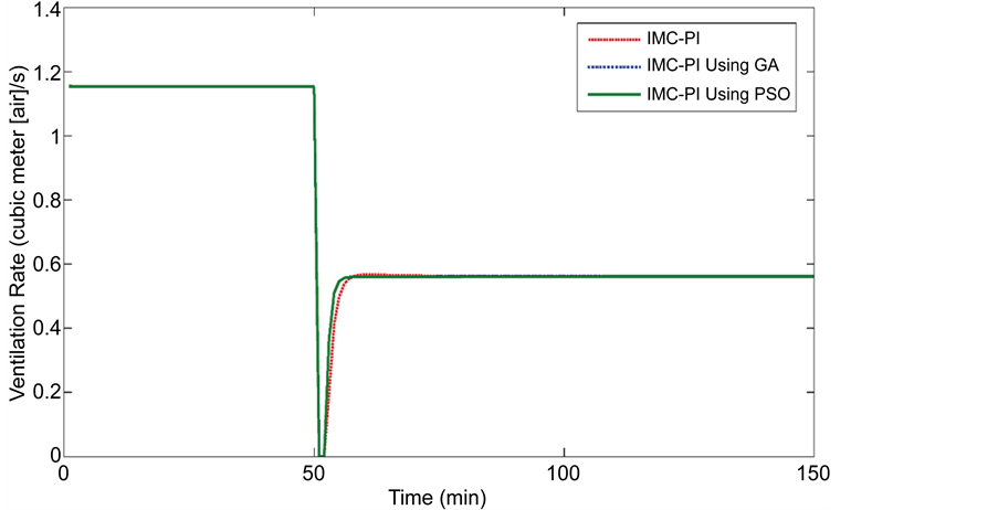
The corresponding variation in control signals namely the ventilation rate and water capacity of the fog system, for the linearized and decoupled model of the GHS are shown in Figure 4(a) and Figure 4(b), respectively. It is observed that the variation in the manipulated variable is smooth.
 (a)
(a) (b)
(b)
Figure 4. Corresponding variations in control signal for servo operations. (a) Variation of ventilation rate with respect to time; (b) Variation of water capacity of fog system with respect to time.
It is observed that the variation in the manipulated variable is smooth.
4.2. Regulatory Operation
4.2.1. For Disturbance in Temperature Loop
Regulatory responses for the three types of IMC-PI controllers are obtained by providing a load change of 5% at time t = 100 minutes on the temperature loop, and the variations observed in temperature and humidity are shown in Figure 5(a) and Figure 5(b), respectively.
 (a)
(a) (b)
(b)
Figure 5. Comparison of closed loop performances of 3 types of IMC-PI controller’s regulatory operation (for disturbances in temperature loop). (a) Variation in temperature for disturbance in temperature loop; (b) Variation in humidity for disturbance in temperature loop.
It is observed that the performance of the IMC-PI controller tuned using PSO is better. This is reflected in the value of λ that is computed using the PSO-based optimization algorithm.
4.2.2. Control Signals (for Disturbance in Temperature Loop)
The corresponding variations in control signals, namely, the ventilation rate and water capacity of the fog system, for the linearized and decoupled model of GHS for a disturbance in the temperature loop at time t = 100 minutes are shown in Figure 6(a) and Figure 6(b), respectively.
 (a)
(a) (b)
(b)
Figure 6. Corresponding variation in control signal for regulatory operation (for disturbance in temperature loop). (a) Variation for ventilation rate for disturbance in temperature loop; (b) Variation of water capacity of fog system for disturbance in temperature loop.
It is observed that the variation in the manipulated variable is smooth.
4.2.3. For Disturbance in Humidity Loop
Regulatory responses for the three types of IMC-PI controllers are obtained by providing a load change of 5% at time t = 100 minutes on the humidity loop and the variations are shown in Figure 7(a) and Figure 7(b) respectively.
 (a)
(a) (b)
(b)
Figure 7. Comparison of closed loop performances of 3 types of IMC-PI controller’s regulatory operation (for disturbances in humidity loop). (a) Variation in temperature for disturbance in humidity loop; (b) Variation in humidity for disturbance in humidity loop.
It is observed that the IMC-PI controller tuned using PSO has the minimum overshoot.
4.2.4. Control Signals (for Disturbance in Humidity Loop)
The corresponding variations in the control signals, namely, the ventilation rate and water capacity of the fog system, for the linearized and decoupled model of GHS for a disturbance in the humidity loop at time t = 100 minutes is shown in Figure 8(a) and Figure 8(b), respectively.
 (a)
(a) (b)
(b)
Figure 8. Corresponding variation in control signal for regulatory operation (for disturbance in humidity loop). (a) Variation of ventilation rate for disturbance in humidity loop; (b) Variation of water capacity of fog system for disturbance in humidity loop.
It is observed that the variation in the manipulated variable is smooth.
5. Quantitative Comparison
The performance measures for IMC-PI controller, IMC-PI tuned using Genetic Algorithm (GA) and IMC-PI tuned using Particle Swarm Optimization (PSO) for linearized and decoupled model of GHS are carried out using the Integral Absolute Error (IAE) and the Integral Square Error (ISE) as given in Equations (14) and (15) respectively.
 (14)
(14)
 (15)
(15)
The performance measures obtained for servo and regulatory operation (for disturbance in temperature loop and for disturbance in humidity loop) are tabulated in Tables 6-11 respectively. From tables it is observed that the error is minimum for the IMC-PI tuned using PSO when compared to IMC-PI using GA and conventional PI.
Table 6. Comparison of performance measures for servo response for Temperature.
Table 7. Comparison of performance measures for servo response for Humidity.
Table 8. Comparison of performance measures for regulatory response for Temperature (for disturbance in temperature loop).
Table 9. Comparison of performance measures for regulatory response for Humidity (for disturbance in temperature loop).
Table 10. Comparison of performance measures for regulatory response for Temperature (for disturbance in humidity loop).
Table 11. Comparison of performance measures for regulatory response for Humidity (for disturbance in humidity loop).
From these closed loop simulation studies, it is seen that IMC-PI controller tuned using Particle Swarm Optimization (PSO) gives better performance than IMC-PI controller using Genetic Algorithm (GA) and IMC-PI controller.
6. Conclusion
In this work, a model based on feedback-feed-forward linearization and decoupling for the GHS has been developed in order to avoid the interactions among the process variables. The IMC based PI controller is designed for the GHS. The controller settings are also tuned using Genetic Algorithm (GA) and Particle Swarm Optimization (PSO) to achieve minimum Integral Square Error (ISE). The results implicate that PSO based IMC-PI controller provides better performance compared to conventional PI and IMC-PI tuned using Genetic Algorithm (GA). Such a control scheme when used for GHS would result in better yield in the production of crops such as tomato, lettuce and broccoli.
Cite this paper
Manonmani, A., Thyagarajan, T., Sutha, S. and Gayathri, V. (2016) Design of Soft Computing Based Optimal PI Controller for Greenhouse System. Circuits and Systems, 7, 3431-3447. http://dx.doi.org/10.4236/cs.2016.711292
References
- 1. Albright, L.D., Gates, R.S., Arvanitis, K.G. and Drysdale, A. (2001) Environmental Control for Plants on Earth and in Space. IEEE Control System Magazine, 21, 28-47.
http://dx.doi.org/10.1109/37.954518 - 2. Pasgianos, G.D., Arvanitis, K.G., Polycarpou, P. and Sigrimis, N. (2003) A Nonlinear Feedback Technique for Greenhouse Environmental Control. Computers and Electronics in Agriculture, 40, 153-177.
http://dx.doi.org/10.1016/S0168-1699(03)00018-8 - 3. Fourati, F. and Chtourou, M. (2007) A Greenhouse Control with Feed-Forward and Recurrent Neural Networks. Simulation Modelling Practice and Theory, 15, 1016-1028.
http://dx.doi.org/10.1109/37.954518 - 4. He, F. and Ma, C. (2010) Modeling Greenhouse Air Humidity by Means of Artificial Neural Network and Principal Component Analysis. Computers and Electronics in Agriculture, 71S, S19-S23.
http://dx.doi.org/10.1016/j.compag.2009.07.011 - 5. Trejo-Perea, M., Herrera-Ruiz, G., Rios-Moreno, J., Miranda, R.C. and Rivas-Arazia, E. (2009) Greenhouse Energy Consumption Prediction Using Neural Networks Models. International Journal of Agriculture and Biology, 11, 1-6.
- 6. Hu, H.G., Xu, L.H., Wei, R.H. and Zhu, B.K. (2011) Multi-Objective Optimization for Greenhouse Environment Using Evolutionary Algorithms. Sensors, 11, 5792-5807.
http://dx.doi.org/10.3390/s110605792 - 7. Cao, Y.J. and Wu, Q.H. (1999) Teaching Genetic Algorithm Using Matlab. International Journal of Electrical Engineering, 36, 139-153.
http://dx.doi.org/10.7227/IJEEE.36.2.4 - 8. Liu, W.K. and Juang, J.G. (2004) Application of Genetic Algorithm Based on System Performance Index on PID Controller. Proceedings of the Ninth Conference on Artificial Intelligence and Application.
- 9. Hasni, A. and Taibi, R. (2011) Optimization of Greenhouse Climate Model Parameters Using Particle Swarm Optimization and Genetic Algorithms. Energy Procedia, 6, 371-380.
http://dx.doi.org/10.1016/j.egypro.2011.05.043